1. Introduction

System identification involves the theory and techniques used to explore and develop mathematical models of static and dynamic systems based on observation data [1, 2]. These systems can be linear, bilinear, or nonlinear [3, 4], with nonlinear systems frequently appearing in industrial applications. As a result, the need for effective modeling techniques for these systems has grown significantly in fields such as signal processing, system analysis, and control. Bilinear models, in particular, are advantageous for industrial applications, as they more accurately capture the nonlinear characteristics of systems compared to linear models. This capability makes them essential in various industrial processes, including heat exchangers, nuclear reactors, and chemical operations.

Some classical identification methods have been applied in the parameter estimation of bilinear systems. For instance, gradient identification techniques have been developed by minimizing criterion functions through negative gradient search [5, 6]. An et al. [8] proposed a multi-innovation gradient-based iterative algorithm for parameter estimation. Additionally, a maximum likelihood multi-innovation stochastic gradient algorithm was proposed for bilinear systems affected by colored noise. Least squares methods are foundational for identifying linear-parameter systems and have been widely utilized across various fields. In prior research, we presented a least squares-based iterative (LSI) algorithm to estimate unknown system parameters [9].

Recently, several new ideas, theories, and principles have emerged in system identification for constructing mathematical models and determining model parameters. Notable among these are the multi-innovation identification theory, hierarchical identification principle, and filtering identification concept, all of which contribute to the advancement of system identification. The multi-innovation identification theory enhances the accuracy of estimating parameters. The hierarchical identification principle significantly improves the computational efficiency of identification algorithms, particularly for large-scale complex systems. Meanwhile, the filtering identification concept addresses parameter estimation challenges in systems with colored noise, thereby enhancing estimation accuracy. These approaches are applicable to bilinear systems. Recently, An et al. [10] explored various parameter estimation algorithms for bilinear systems utilizing the maximum likelihood gradient-based iterative and hierarchical principles. Additionally, Gu examined an identification algorithm based on multi-innovation stochastic gradient that incorporates filtering methods for bilinear systems utilizing data filtering theory [11].

The Newton method, a classical optimization tool, is a root-finding algorithm that leverages the initial terms of a function's Taylor series expansion near an estimated root [12]. This method has been extensively studied over the years and has diverse applications, including minimization and maximization problems, solving transcendental equations, and numerically verifying solutions to nonlinear equations. For instance, Xu introduced a separable Newton recursive algorithm based on dynamically discrete measurements, which utilizes system responses with progressively increasing data lengths [13].

Notably, bilinear systems pose a greater challenge than general linear ones due to the increased number of parameters that need to be estimated. This complexity makes standard parameter estimation methods inadequate for achieving high-precision estimates. Additionally, the characteristics of bilinear systems prevent the direct application of conventional state estimation techniques like Kalman filtering [14, 15, 16] and finite impulse response (FIR) filter [17]. Consequently, there is a need to develop a novel state estimator utilizing Kalman filtering, specifically tailored and modified to meet the unique requirements of bilinear systems [18].

In this paper, we present a novel identification algorithm aimed at identifying bilinear stochastic systems. Our approach introduces a Newton-based iterative algorithm for parameter estimation. Subsequently, we employ the bilinear state observer-based NI (BSO-NI) method to achieve simultaneous estimation of states and parameters. The availability of the scheme is validated by comparing estimation errors with those of gradient-based algorithms. Below, we summarize the main contributions of our work.

2. System description

Focus on a bilinear system in state-space representation featuring autoregressive noise, described by an observability canonical model:

where $𝒙\left(t\right)\in m^{}$, $y\left(t\right)\in$, and $u\left(t\right)\in$ are the state vector, output and input variable, and $𝑨\in {m\times m}^{}$, $𝑩\in {m\times m}^{}$, $𝑪\in m^{}$, and $𝑫\in {1\times m}^{}$ are the matrices/vectors of the system parameters:

where ${𝑰}_{m-1}$ represents an identity matrix of size $\left(m-1\right)\times \left(m-1\right)$, $w\left(t\right)$ is the process noise, $v\left(t\right)$ is the measurement noise, let the known dimension of the state vector be $m$, and assume that $y\left(t\right)=0$ and $v\left(t\right)=0$ for $t⩽0$. Bilinear systems can be interpreted as linear systems with time-varying characteristics, exhibiting stability that changes over time. The stability of these systems is determined by the time-varying matrix $𝑨+𝑩u\left(t\right)$. By designing an input sequence that ensures all eigenvalues of $𝑨+𝑩u\left(t\right)$ remain below 1.

Based on Equations (1)–(6), the subsequent relationships exist:

where $p=1,\cdots ,m-1$. To multiply both sides of Equation (7) by $z^{-p}$, and sum from $p=1$ to $p=m-1$, and then add this to Equation (8), where both sides are multiplied by $z^{-m}$, one can derive

Inserting (9) into (2) gives:

After that, one define the parameter vector $𝜽$, along with the data vector $𝝋\left(t\right)$ as:

The expression for $y\left(t\right)$ in Equation (11) can be expressed as follows:

The model for identification is established in Equation (18). The information vector $𝝋\left(t\right)$ includes $𝒙\left(t-l\right)$$\left(l=1,2,\cdots ,m\right)$, $u\left(t-l\right)$, and the system parameters $a_l$, ${𝒃}_l$, $c_l$ which together form the parameter vector $𝜽$. The goal of this study is to explore novel approaches for estimating these states and parameters using $\left\{u\left(t\right)\right\}$, $\left\{y\left(t\right)\right\}$, which is affected by white noise $v\left(t\right)$. Equation (18) serves as the basis for deriving the iterative estimation approach.

3. The NI algorithm for parameter estimation

Parameter estimation for different types of systems has been tackled using stochastic gradient methods, iterative methods based on gradients, and various other gradient-based approaches [19]. In order to enhance the precision of parameter estimation further, the use of Newton search has been suggested. Based on the iterative identification idea, a Newton iterative (NI) algorithm has been developed specifically for bilinear systems.

Considering the data length $h$, we define the criterion function

where the stacked observed data $𝒀\left(h\right)$ and the stacked information matrix $𝚽\left(h\right)$ are defined as:

Calculating the partial derivative of $J_1\left(𝜽\right)$ in relation to $𝜽$ produces

Define ${\widehat{𝜽}}_k$ as the approximation of $𝜽$ during iteration $k$, where $k=1,2,3,\cdots$ represents an iterative parameter. Set the estimate of the stacked information matrix $𝚽\left(h\right)$ at iteration $k$ as follows:

where

From Equation (1), we can calculate the gradient of $J_1\left(𝜽\right)$ at $𝜽={\widehat{𝜽}}_{k-1}$:

The gradient method relies on the first derivative, whereas the Newton method exhibits quadratically convergence. To enhance the accuracy of parameter estimation, we calculate the second partial derivative of the criterion function $J_1\left(𝜽\right)$ with respect to $𝜽$, resulting in the Hessian matrix

Using the Newton search and iterative identification idea to minimize $J_1\left(𝜽\right)$, we can obtain the following iterative relation of computing $𝜽$:

Substituting (11) into the above equation, we obtain:

From Equations (3)–(15), we can summarize the Newton iterative (NI) algorithm for the bilinear stochastic systems as follows:

In the above NI algorithm for the parameter estimation, we assume that the system states in the information vector are known. Thus, we design the state estimator to estimate them.

4. Bilinear state observer based NI algorithm

Let $𝒙𝒊\left(t\right):=𝑩𝒙\left(t\right)+𝑪$. This type of bilinear state-space framework can be represented in the form of a linear time-varying model:

According to the NI algorithm, the obtained parameter estimates ${\hat{a}}_{l,k}$, ${\widehat{𝒃}}_{l,k}$ and ${\hat{c}}_{l,k}$ from ${\widehat{𝜽}}_k$ can be used to construct the estimates ${\widehat{𝑨}}_k$, ${\widehat{𝑩}}_k$ and ${\widehat{𝑪}}_k$ of the system matrices/vector $𝑨$, $𝑩$ and $𝑪$, respectively. According to the Kalman filtering principle and referencing to [7], we can design the bilinear state estimator as follows:

Equations (3)–(11) form the state estimator for bilinear systems, enabling the computation of the state estimation vector denoted by ${\widehat{𝒙}}_k\left(t\right)$. The initial values ${\widehat{𝒙}}_k\left(1\right)$ and ${𝑷}_k\left(1\right)$ can be chosen arbitrarily. For instance, we can set ${\widehat{𝒙}}_k\left(1\right)={\mathrm{𝟏}}_m$ and ${𝑷}_k\left(1\right)={𝑰}_m$.

Based on the above preparations, Equations (17)–(26) and (3) to (11) form the bilinear state estimator-based NI (BSO-NI) algorithm, and the joint state and parameter estimation is realized. Here, we can summarize the BSO-NI algorithm in Algorithm 1:

5. Bilinear state estimator based GI algorithm

To highlight the advantages of the proposed BSO-NI algorithm, this section presents the bilinear state observer based GI (BSO-GI) algorithm for comparison.

When the measurement data are collected from the system outputs, it is important to utilize these data effectively to update the parameter estimates [20]. Consider the $𝒀\left(h\right)$ and the $𝚽\left(h\right)$ defined in Section 3. Utilizing negative gradient search [21] and minimizing $J_1\left(𝜽\right)$ get

where the iterative step-size ${\mu }_k$ satisfies

Nevertheless, similar issues occur. The information matrix $𝚽\left(h\right)$ includes the unknown terms $x_i\left(t-m\right)$ and $𝒙\left(t-i\right)$. Following the similar method from the BSO-NI algorithm, we replace these unknowns with their estimates ${\hat{x}}_{i,k}\left(t-m\right)$ and ${\widehat{𝒙}}_k\left(t-i\right)$. Following this, we can derive the estimated information matrix ${\widehat{𝚽}}_k\left(h\right)$. By substituting the unknown information matrix $𝚽\left(h\right)$ in (1) with its estimate ${\widehat{𝚽}}_k\left(h\right)$, and referring to the bilinear state estimator in (3)–(11), the BSO-GI algorithm for bilinear systems, based on BSO, can be outlined as follows:

Equations (3)–(24) form the BSO-GI algorithm. The algorithmic procedure for bilinear systems are outlined below:

6. Simulations

The following consider a second-order bilinear system defined by the equations:

The system parameters will be estimated are

For the simulation, the sequence $\left\{u\left(t\right)\right\}$ is set as an independent persistent excitation signal that has a mean of zero and unit variance, while $\left\{v\left(t\right)\right\}$ is modeled as a white noise sequence, exhibiting zero mean and variances ${\sigma }^2={0.50}^2$, ${\sigma }^2={1.00}^2$ and ${\sigma }^2={1.50}^2$, respectively. We define $h$ as 500 for the data length and establish a maximum of 30 iterations, represented by $k_{\max }$.

Figure 1 The estimation errors $\delta$ versus $k$ for the BSO-NI and BSO-GI algorithms.

Figure 2 The $𝑨$ vector parameter estimates versus $k$ for the BSO-NI and BSO-GI algorithms.

Figure 3 The $𝑩$ matrix parameter estimates versus $k$ for the BSO-NI and BSO-GI algorithms.

Figure 4 The $𝑪$ vector parameter estimates versus $k$ for the BSO-NI and BSO-GI algorithms.

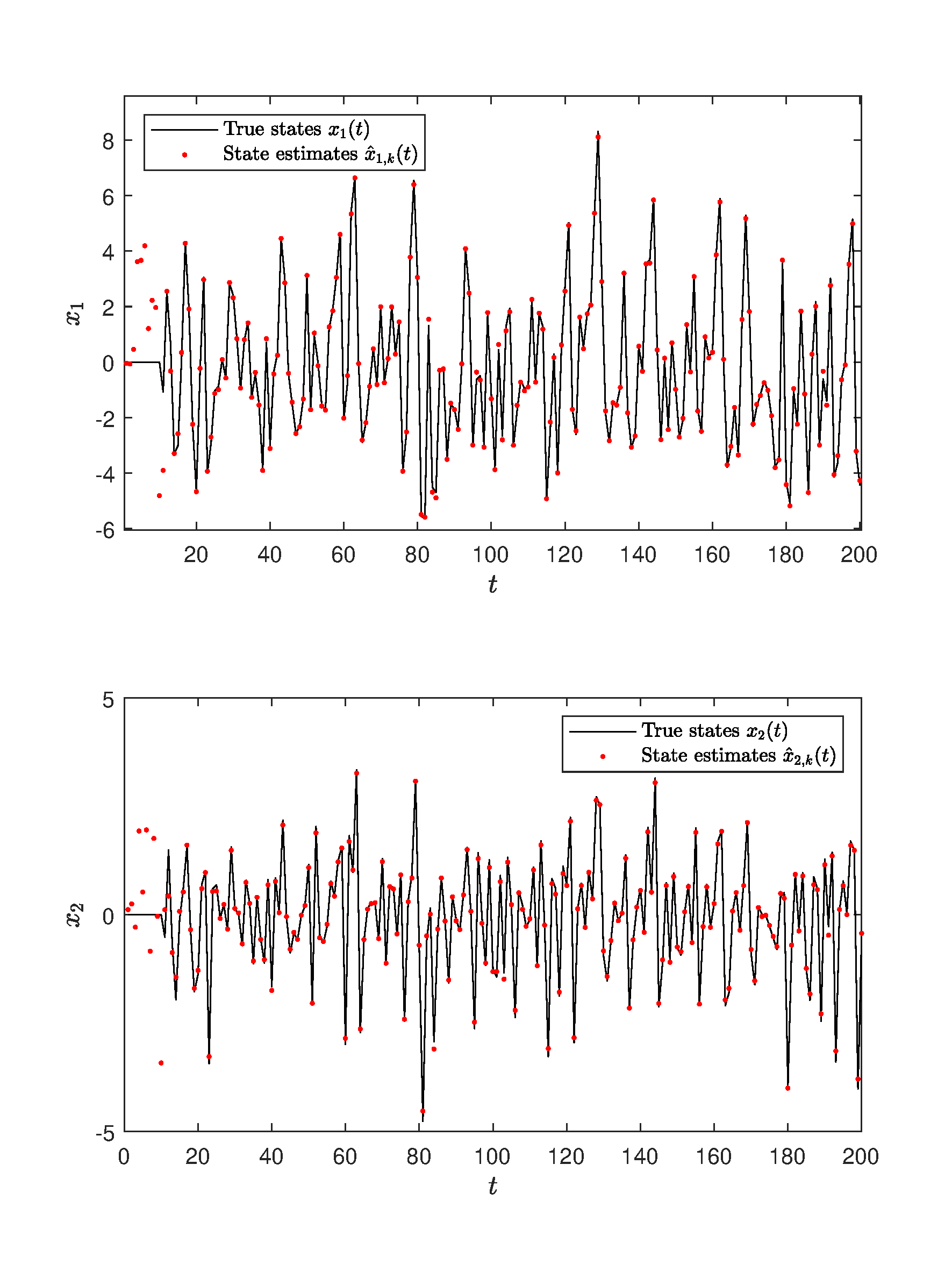
For the state estimation of this bilinear system, the BSO-NI algorithm is utilized to estimate each state. The true state values and the state estimates are shown in Figure 5. With the length of the data increasing, the state estimates tend toward the actual values.

Figure 5 The true states and their estimates for the BSO-NI algorithm.

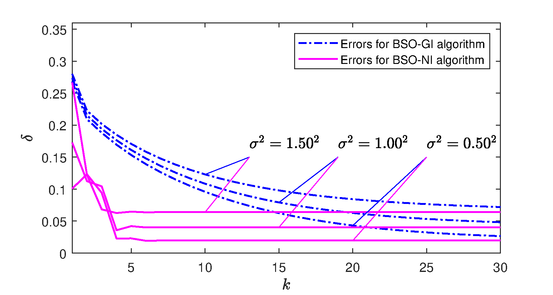
Apply the BSO-NI algorithm Equations (17)–(26) and Equations (3)–(11) to estimate the parameters $𝜽$ and the states $𝒙$. For comparison, we also utilize the BSO-GI algorithm Equations (3)–(24) for the bilinear system estimation. The parameter estimation errors $\delta =\Vert {\widehat{𝜽}}_k-𝜽\Vert /\Vert 𝜽\Vert$ for both algorithms are presented in Figure 1. From it, it is evident that the parameter estimation errors $\delta$ gradually decreases with the increase of $k$. Additionally, as the noise levels diminish, both algorithms yield more accurate parameter estimates. Under the same noise conditions, the BSO-NI algorithm demonstrates greater parameter estimation accuracy compared to the BSO-GI algorithm.

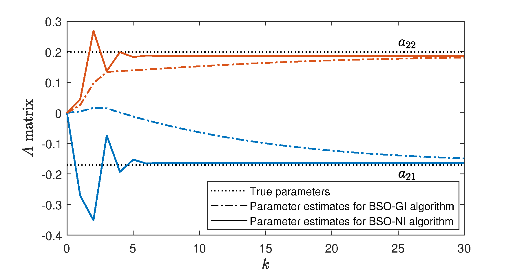
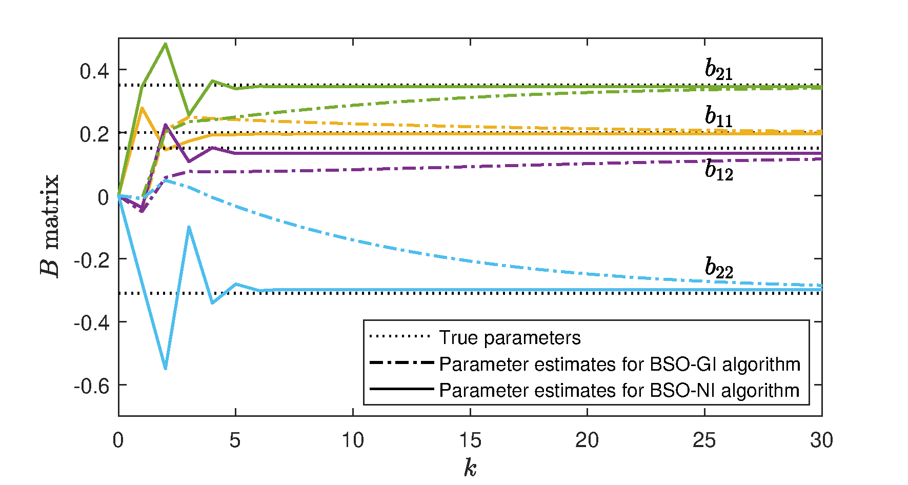
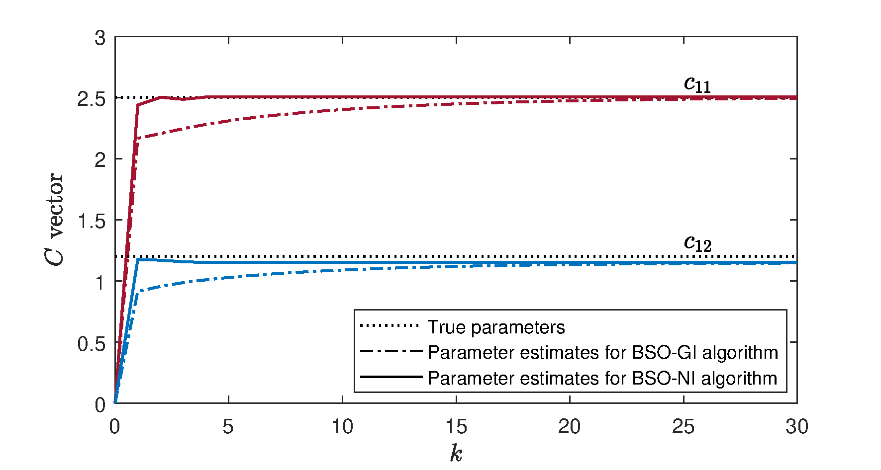
In order to better demonstrate the estimation effect of each parameter for the bilinear system, we use two algorithms to predict each parameter matrix or vector respectively, and show the comparison results in Figures 2–4. Figure 2 shows true parameters and the estimation results of the parameters in the $𝑨$ matrix. Figure 3 displays the parameter estimation values for two algorithms in the $𝑩$ matrix, and the parameter estimates in the $𝑪$ vector are clearly presented in Figure 4. These figures clearly illustrate that the BSO-NI algorithm outperforms the BSO-GI algorithm in terms of parameter estimation precision. Furthermore, the BSO-NI algorithm converges to the parameter estimates more rapidly.

7. Conclusion

This paper studies the combined estimation of states and parameters for bilinear systems. By means of the Newton search and batch data, we derive a Newton iterative (NI) algorithm to estimate the parameters that are not known. Drawing inspiration from the Kalman filtering, the bilinear state estimator (BSO) is created for estimating the unknown states, and a BSO based NI (BSO-NI) algorithm is proposed for the bilinear systems. In comparison to gradient-based algorithm, this NI algorithm achieves higher estimation accuracy. Simulation results illustrate the validity of the suggested method.