3.1 Field data collection

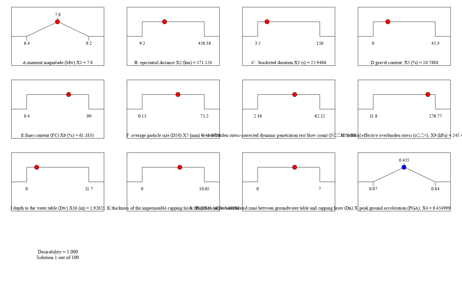
A dataset comprising 234 records was globally compiled from post-earthquake observations, focusing on suspected liquefaction sites characterized by a gravelly soil profile, as documented in prior literature [16]. Each record includes diverse data points, which are the input variables such as the earthquake’s moment magnitude (Mw) represented by $X_1$, epicenter distance (R) denoted as $X_2$ in kilometers, bracketed duration (t) indicated by $X_3$ in seconds, gravel content (G) as $X_5$ in percentage, fines content (F) denoted by $X_6$ in percentage, average particle size (D50) represented by $X_7$ in millimeters, overburden stress-corrected dynamic penetration test blow count (N’120 Blows) indicated by $X_8$, vertical effective overburden stress ($\sigma$’v) represented by $X_9$ in kilopascals (kPa), depth to the water table (Dw) as $X_{10}$ in meters, thickness of the impermeable capping layer (Hn) denoted by $X_{11}$ in meters, and thickness of the unsaturated zone between the groundwater table and capping layer (Dn) as $X_{12}$ in meters. The output is the peak ground acceleration (PGA) measured in gravitational units (g) and represented as $X_4$. The statistical characteristics and the Pearson correlation matrix for the dataset are succinctly conducted and summarized.

3.2 The theoretical framework of the RSM

Figure 1 RSM flow chart of modeling optimization.

Figure 2 The RSM 3D surface framework.

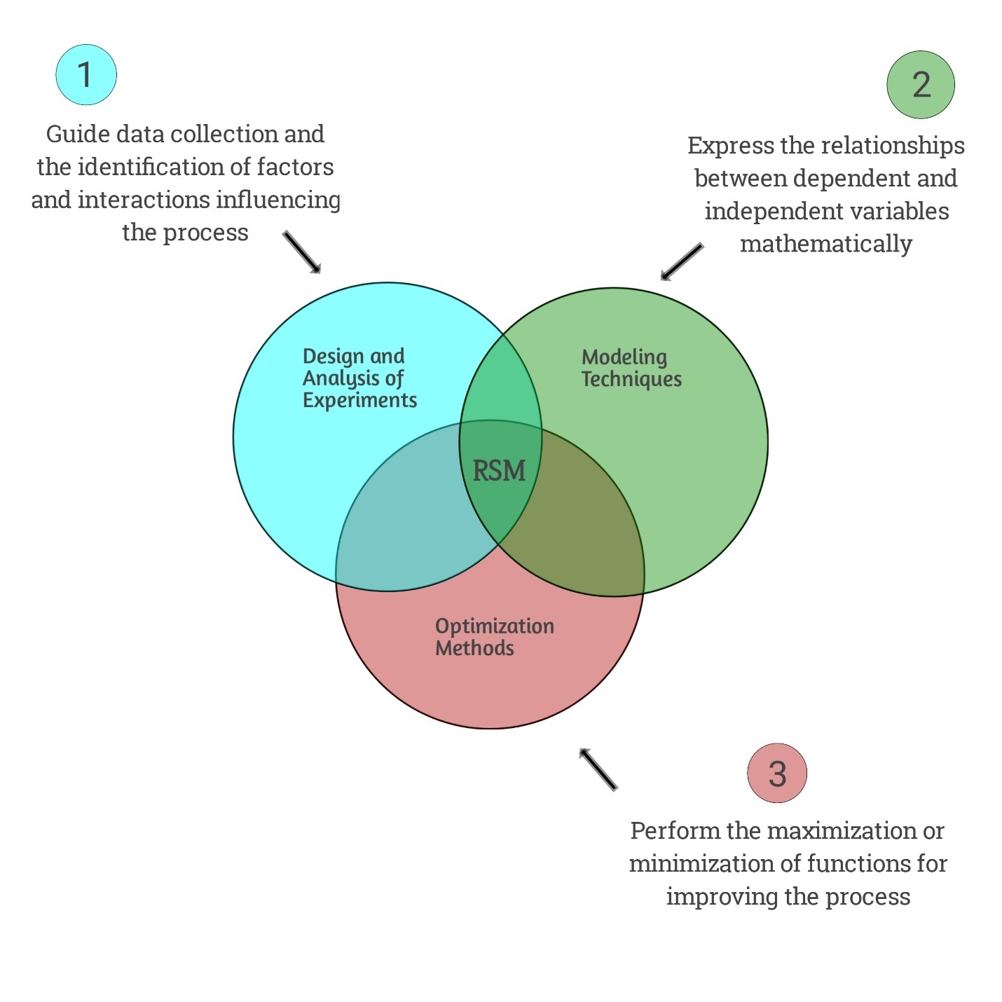
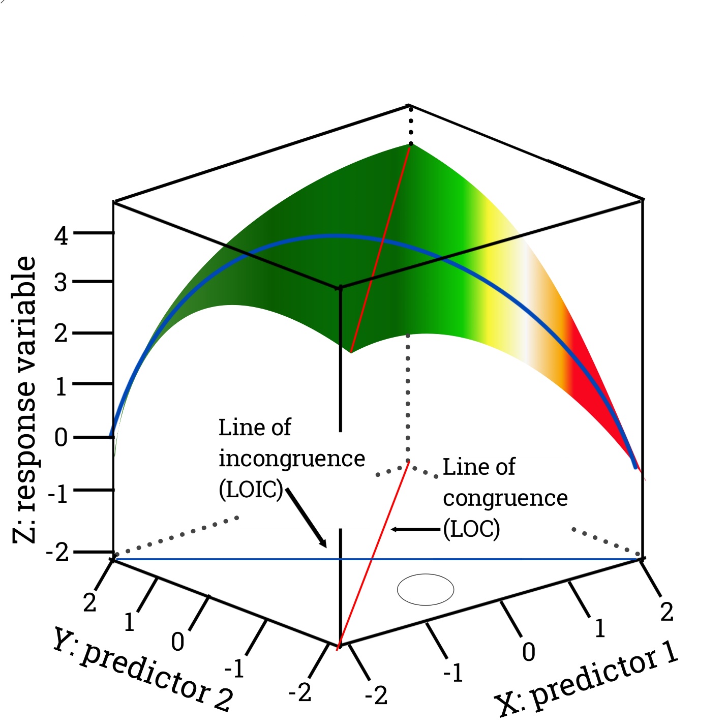
Response Surface Methodology (RSM) is a collection of mathematical and statistical techniques used for modeling and analyzing the relationships between multiple variables and the response of a system [17]. The RSM flow chart of modeling optimization and the 3D surface framework are represented in Figures 1 and 2. It is commonly applied in scientific and engineering fields, particularly in the optimization of complex processes, product development, and quality improvement. RSM is often used to explore and optimize the response of a system within a specific region of the design space. RSM often begins with the design of experiments to systematically collect data on the response of a system as a function of multiple input variables [18]. These experiments are designed to efficiently explore the design space and capture the relationships between inputs and outputs. Using regression analysis and other statistical techniques, mathematical models are developed to represent the relationship between the input variables and the system’s response. These models may include linear, quadratic, and interaction terms to capture the behavior of the system. Once the models are developed, optimization techniques are employed to identify the optimal settings for the input variables that lead to the desired response of the system [19]. This involves finding the input combinations that maximize or minimize the response based on specific criteria. The models developed using RSM are validated to ensure their accuracy and reliability. This may involve conducting additional experiments to confirm the predicted responses based on the optimized input variables. RSM often involves the graphical representation of response surfaces, contour plots, and other visual tools to help understand the relationships between the input variables and the system’s response [20]. Applications of RSM can be found in various fields, including chemical engineering, pharmaceuticals, food science, agriculture, manufacturing, and product development. It is a powerful tool for efficiently optimizing processes and products, reducing experimentation costs, and gaining a deeper understanding of complex systems [18]. Response Surface Methodology (RSM) utilizes mathematical models to characterize and optimize the behavior of complex systems. These models can be classified based on their structure and the nature of the relationships they represent. The linear RSM models describe the relationship between the input variables and the response as a linear function. A simple linear model may include terms for each input variable, while a multiple linear regression model can include interaction terms as well. However, linear models may not always capture the full complexity of a system’s behavior [17]. The Quadratic RSMmodels extend linear models by including squared terms for the input variables. This allows for the representation of nonlinear relationships between variables and the response. Quadratic models are particularly useful for capturing curvature in the response surface. Interaction Models: Interaction models include terms that represent the interaction effects between input variables [20]. These terms capture the combined effect of two or more variables on the response, allowing for the representation of non-additive relationships. The full cubic RSMmodels go beyond quadratic models by including cubic terms for the input variables. These models can capture more complex nonlinear behavior, including inflection points and more pronounced curvatures in the response surface. In addition to the aforementioned models, RSM can incorporate higher-order terms to capture even more complex relationships [19]. This may include models with terms representing higher powers of the input variables, allowing for the representation of highly nonlinear behavior. In cases where the number of input variables is large, fractional factorial designs can be used to construct reduced models that capture the most important effects. These models provide a more efficient way to explore the design space and identify key factors. The selection of the appropriate model type in RSM depends on the nature of the system being studied, the complexity of the relationships, and the available experimental data. Model selection is typically guided by statistical criteria, such as goodness of fit, predictive capability, and the trade-off between model complexity and interpretability [21]. Once a model is selected, it can be used for optimization and prediction within the specified experimental region.

In Response Surface Methodology (RSM), the mathematical formulation involves developing equations to model the relationship between the input variables and the response of a system. The most common form of the mathematical equation used in RSM is the response surface model. This can take different forms based on the complexity of the relationships being studied. Here are the general forms of the mathematical equations used in RSM: Linear Model: The general form of a linear model in RSM with two input variables ($X_1$ and $X_2$) can be expressed as [20]:

where, Y represents the response variable, ${\beta }_0$ is the intercept, ${\beta }_1$ and ${\beta }_2$ are the coefficients for the first and second input variables, $X_1$ and $X_2$, and $\epsilon$ represents the error term. Quadratic Model: A quadratic model extends the linear model by including squared terms for the input variables, and can be expressed as:

where, ${\beta }_{11}$ and ${\beta }_{22}$ represent the coefficients for the squared terms of $X_1$ and $X_2$, and ${\beta }_{12}$ represents the coefficient for the interaction term. Interaction Model: An interaction model includes terms that represent the interaction effects between input variables, and can be expressed as:

where ${\beta }_{12}$ represents the coefficient for the interaction term. Cubic Model: A cubic model extends the quadratic model by including cubic terms for the input variables, and can be expressed as:

In this equation, ${\beta }_{111}$ and ${\beta }_{222}$ represent the coefficients for the cubic terms of $X_1$ and $X_2$. The general response surface model encompasses higher-order terms and can be expressed as a more complex equation that includes linear, quadratic, cubic, and possibly higher-order terms, as well as interaction terms [21]. In the above equations, the $\beta$ coefficients represent the parameters to be estimated from the experimental data, and $\epsilon$ represents the error term. These equations are derived through regression analysis based on the experimental data collected using designed experiments [22]. The selection of the appropriate model is based on the nature of the relationships between the input variables and the response, and is guided by statistical criteria and the complexity of the system under study. However, the general equation for a response surface model (RSM) can be expressed as:

where Y is the predicted response variable, ${\beta }_0$ is the model intercept, ${\beta }_i$, ${\beta }_{ii}$, ${\beta }_{ij}$, etc., are the coefficients for the linear, quadratic, and interaction terms, respectively, $X_i$, $X_{ii}$, $X_{ij}$, etc., are the independent variables (factors) at different levels and $\epsilon$ is the error term. In this equation, the model can include both linear and nonlinear terms to capture the relationship between the independent variables and the response [21]. The coefficients are estimated through methods such as least squares regression, and the model can be used to analyze and optimize processes in fields such as engineering, chemistry, and manufacturing.

4.1 Discussion

As presented in Table 1, apositive predicted $R^2$ of 0.9997 implies that the overall mean may not be a better predictor of the response than the current model. In some cases, a higher-order model may also predict better. Adequate precision measures the signal-to-noise ratio. A ratio greater than 4 is desirable. This shows the PGA model’s ability to navigate the design space for the design of earthquake-induced ground movement events across the world. Adequate precision and navigation of design space are concepts commonly encountered in the context of experimental design and optimization. Adequate precision refers to the level of accuracy and reliability in the measurements and predictions obtained from a given experimental or predictive model. In the context of experimental design, adequate precision implies that the experimental setup and the associated statistical analysis are capable of providing results that are sufficiently accurate and consistent to draw valid conclusions. For predictive models, adequate precision indicates that the model’s predictions are reliable and provide meaningful insights on the design space navigation. Design space refers to the range of input variables or parameters that can be manipulated within a given system or process. Navigation of design space involves exploring and understanding the relationships between input variables and their effects on the output or response of interest. It often involves the use of techniques such as response surface methodology, design of experiments, optimization algorithms, and sensitivity analysis to systematically explore the design space, identify influential factors, and optimize the system’s performance. In practice, achieving adequate precision and effectively navigating the design space are critical for conducting meaningful experiments, developing accurate predictive models, and optimizing processes or products in various fields such as engineering, manufacturing, and scientific research. These concepts are fundamental to the successful implementation of methodologies aimed at understanding and improving complex systems. The present model’s adequate precision ratio is 11.158, which indicates an adequate signal. This model, however, can be used to navigate the design space.

Figure 3 Normal RSM plot of residuals.

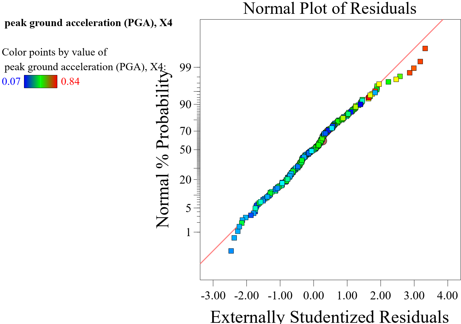
In the context of a response surface model (RSM), a normal plot of residuals presented in Figure 3 is a graphical tool used to assess the assumption of normality for the residuals of the model. The normal plot, also known as a normal probability plot, is a diagnostic tool that helps to determine whether the residuals follow a normal distribution, which is a key assumption for many statistical analyses. Interpreting a normal plot of residuals for an RSM model involves examining how the points on the plot align with the diagonal line, which represents a theoretical normal distribution. If the points on the normal plot approximately form a straight line that closely follows the diagonal line, it suggests that the residuals are approximately normally distributed as shown. This alignment indicates that the normality assumption in the prediction of the PGA is reasonable, supporting the validity of the statistical inferences drawn from the model. But if the points on the normal plot had deviated substantially from the diagonal line, showing a pronounced curvature or systematic departure from linearity, it may indicate non-normality in the residuals. This could imply issues such as skewness, heavy tails, or other departures from the normal distribution. Additionally, the normal plot can reveal information about the presence of outliers or heavy tails in the residuals. Outliers may appear as points that deviate significantly from the expected pattern on the plot, providing insights into potential influential observations. Ultimately, the normal plot of residuals serves as a visual aid for assessing the distributional assumptions of the residuals in an RSM model. Deviations from the expected pattern in the plot can prompt further investigation into the adequacy of the model and potential improvements, such as exploring alternative modeling techniques or identifying influential data points.

Figure 4 RSM plot of residuals versus predicted PGA values.

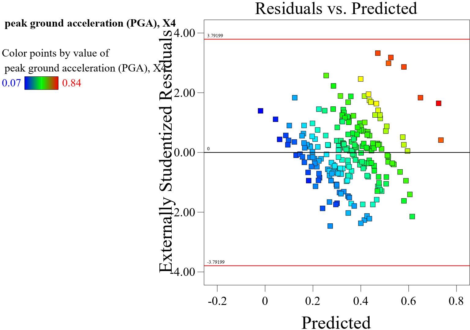
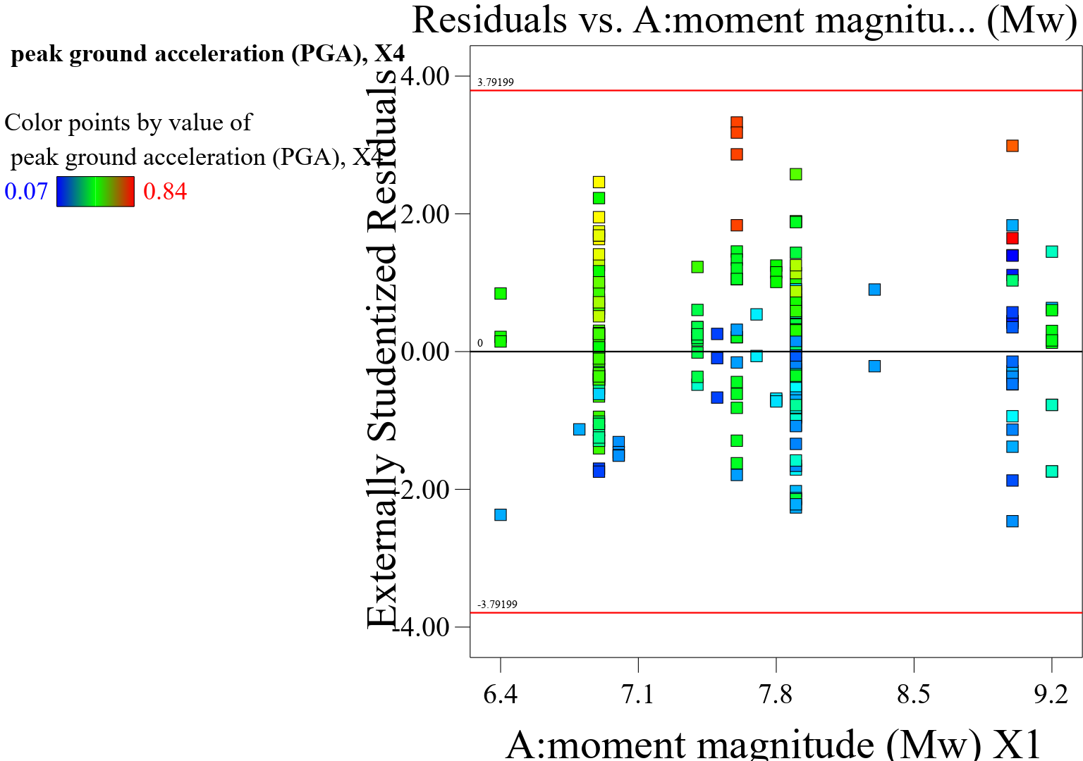
The plot of residuals versus predicted values illustrated in Figure 4 in a response surface model (RSM) is a diagnostic tool used to assess the appropriateness of the model and to detect potential patterns or trends in the residuals. Ideally, the plot should exhibit a random scatter of points around the horizontal line at zero. This indicates that the residuals are not systematically related to the predicted values, suggesting that the model’s assumptions are being met. If the plot shows discernible patterns, such as a systematic increase or decrease in the residuals as the predicted values change, it may indicate potential issues with the model. For example, if the residuals tend to increase or decrease as the predicted values increase, this could suggest that the model is missing important terms or has a non-linear relationship with the response. Patterns in the spread of residuals at different predicted values can also be indicative of heteroscedasticity, where the variability of the residuals changes across the range of predicted values. This can be a concern as it violates the assumption of homoscedasticity, which assumes that the variance of the residuals is constant across the range of predicted values. The plot can also help identify potential outliers or influential data points that have a large impact on the model’s performance. Outliers may appear as points that deviate significantly from the expected random scatter, potentially warranting further investigation. Overall, the plot of residuals versus predicted values serves as a valuable diagnostic tool for assessing the adequacy of the RSM model. It helps in identifying potential model misspecification, non-linearity, heteroscedasticity, and influential observations. In summary, the plot of residuals versus predicted values provides insights into the performance and appropriateness of the RSM model, helping to identify areas where the model may need improvement or where further investigation is warranted.

Figure 5 RSM plot of residuals versus field run of PGA values.

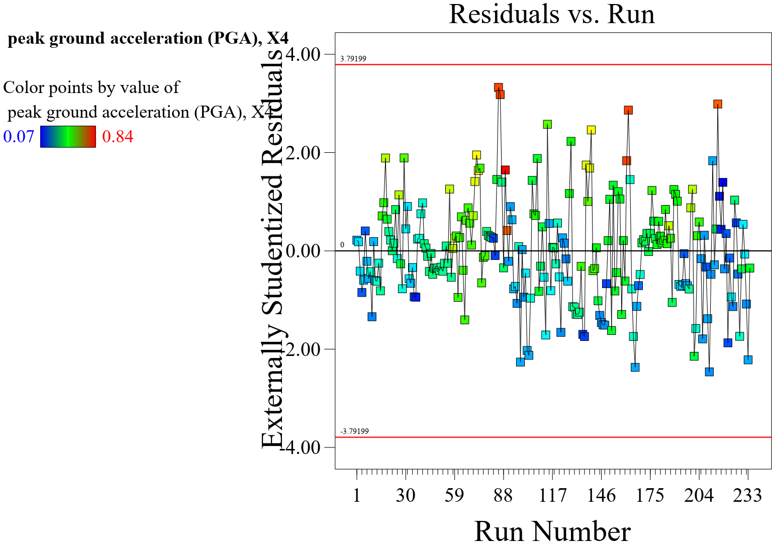
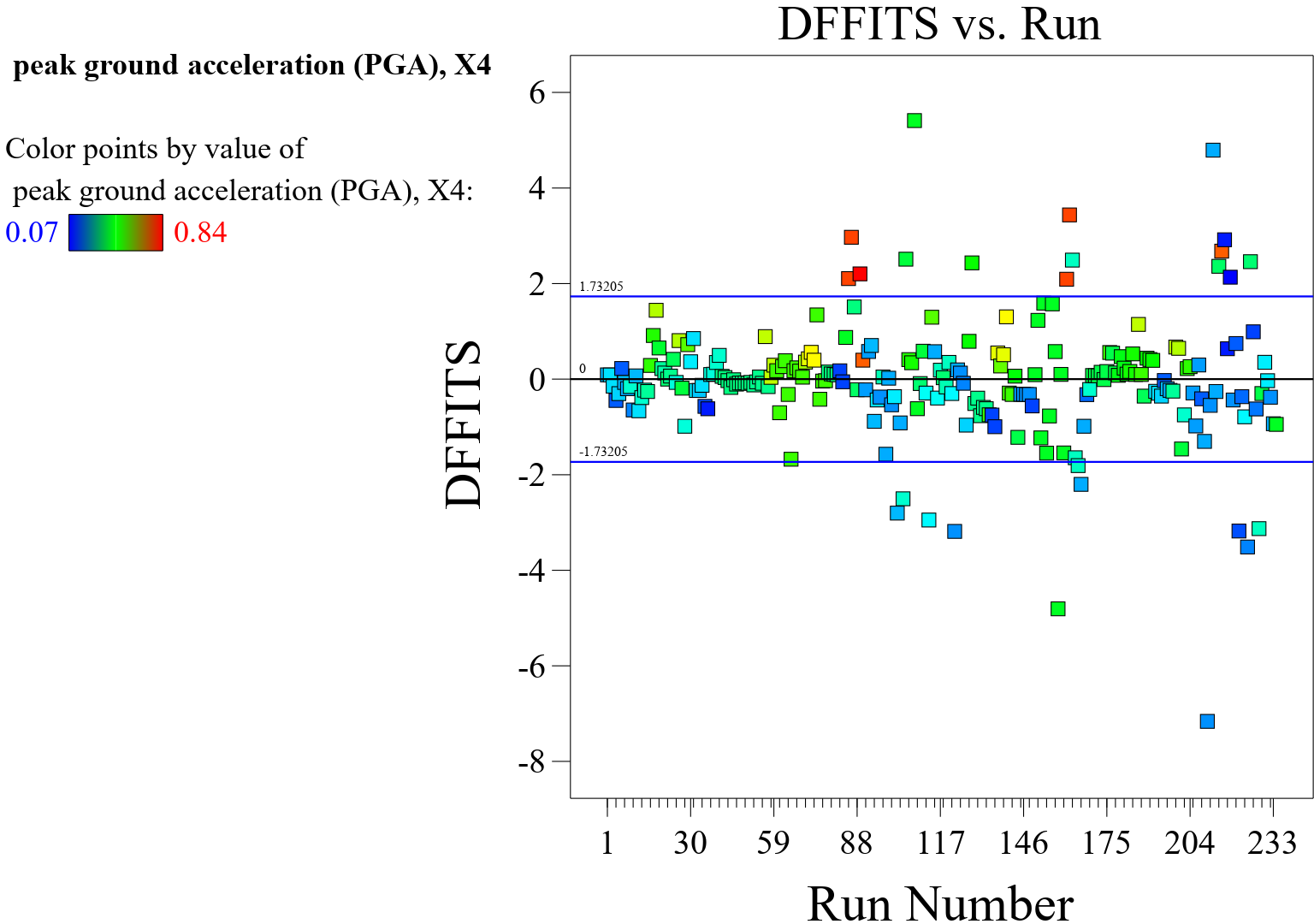
The plot of residuals versus experimental run values presented in Figure 5 in a response surface model (RSM) is a diagnostic tool used to assess the quality and appropriateness of the model. It helps in identifying potential patterns or trends in the residuals with respect to the experimental run values. Ideally, the plot should exhibit a random scatter of points around the horizontal line at zero. This indicates that the residuals are not systematically related to the experimental run values, suggesting that the model’s assumptions are being met. If the plot shows discernible patterns, such as a systematic increase or decrease in the residuals as the experimental run values change, it may indicate potential issues with the model. For example, if the residuals tend to increase or decrease as the experimental run values increase, this could suggest that the model is missing important terms or has a non-linear relationship with the response. Patterns in the spread of residuals at different experimental run values can also be indicative of heteroscedasticity, where the variability of the residuals changes across the range of experimental run values [23]. This can be a concern as it violates the assumption of homoscedasticity, which assumes that the variance of the residuals is constant across the range of experimental run values. The plot can help identify potential outliers or influential data points that have a large impact on the model’s performance. Outliers may appear as points that deviate significantly from the expected random scatter, warranting further investigation. Overall, the plot of residuals versus experimental run values serves as a valuable diagnostic tool for assessing the adequacy of the RSM model. It helps in identifying potential model misspecification, non-linearity, heteroscedasticity, and influential observations. In summary, the plot of residuals versus experimental run values provides insights into the performance and appropriateness of the RSM model, helping to identify areas where the model may need improvement or further investigation.

Figure 6 RSM plot of Cook’s distance on PGA prediction.

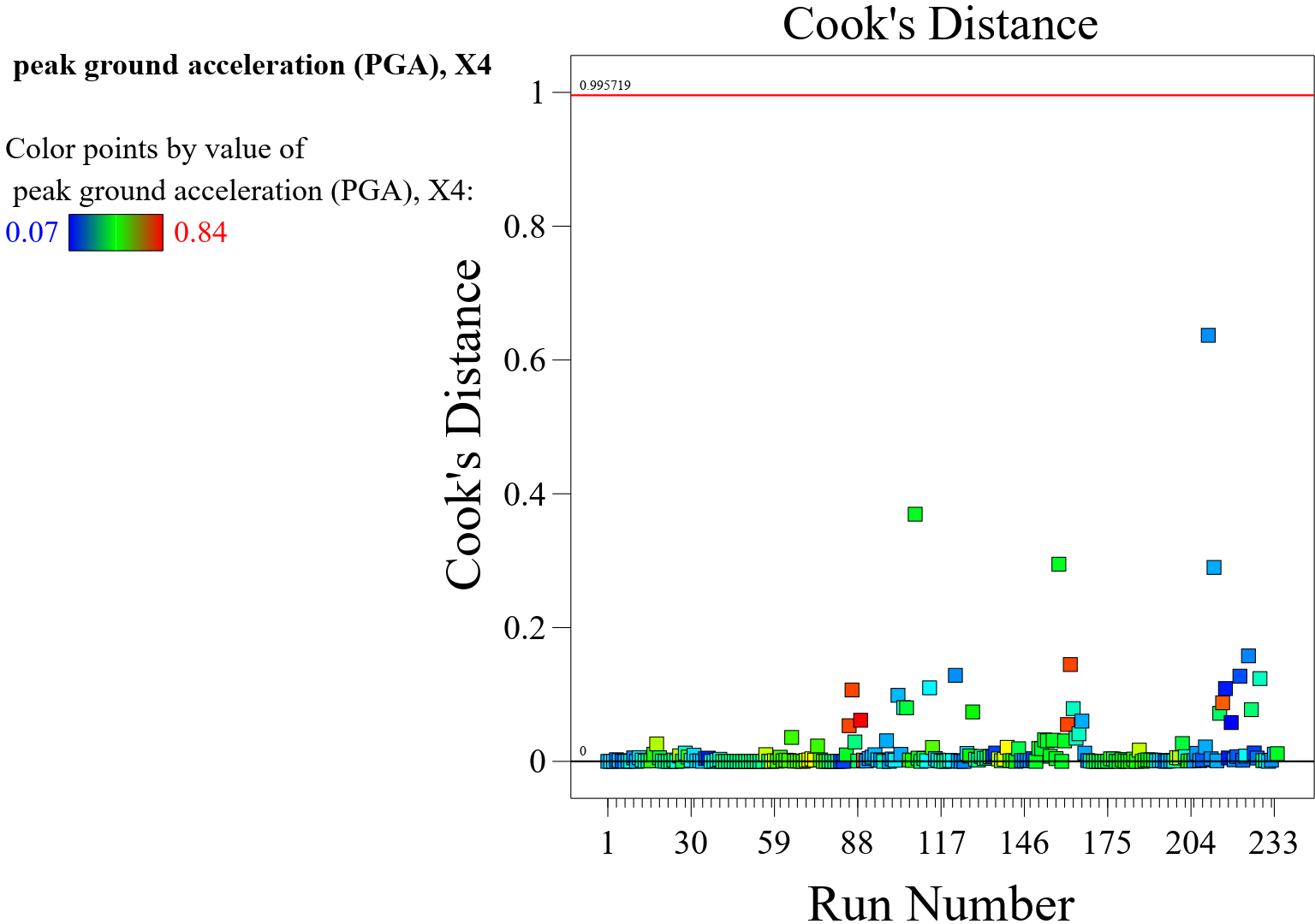
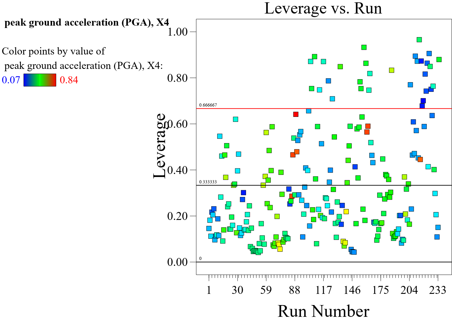
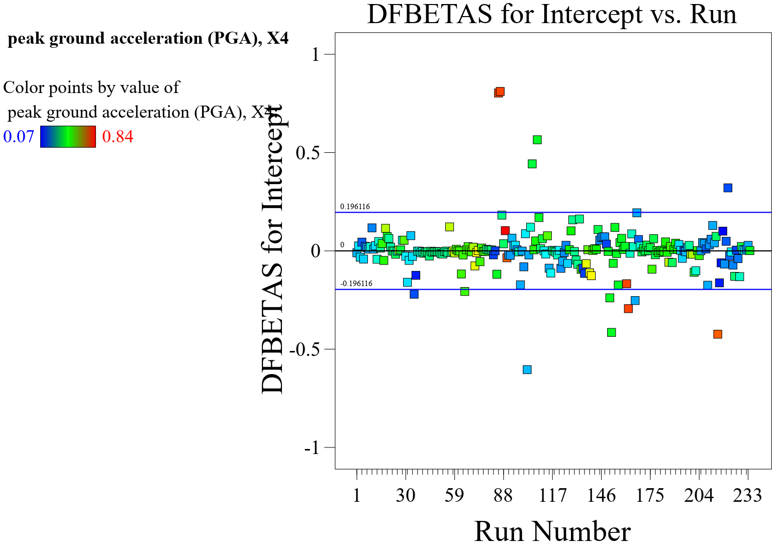
In the context of a response surface model (RSM), Cook’s distance illustrated in Figure 6 is a measure used to identify influential data points that have a disproportionately large impact on the estimated coefficients of the model. It is a useful diagnostic tool for detecting influential observations, which, if left unaddressed, can significantly affect the model’s fit and predictions. Observations with large Cook’s distances are considered influential, meaning they have a strong influence on the model’s coefficients. In the plot, influential points are typically represented by data points with high Cook’s distances, often plotted above a certain threshold line. Large Cook’s distances indicate that certain observations may substantially affect the model’s fit and predictions. These observations may have a notable impact on the estimated coefficients and can potentially distort the overall model performance. When reviewing the plot of Cook’s distance, researchers can use it as a guide for deciding whether to take corrective actions, such as potentially removing influential observations, transforming variables, or considering alternative modeling approaches to address the impact of these points. Interpretation of Cook’s distance should take into account the specific context of the data and the goals of the analysis. In some cases, influential observations may be an essential part of the dataset, and removing them may not be appropriate without careful consideration of the underlying reasons for their influence. In summary, the plot of Cook’s distance in an RSM model provides valuable insights into influential observations that may have a significant impact on the model’s coefficients and predictive performance. It serves as a diagnostic tool to guide decisions related to model adjustments and the treatment of influential data points.

Figure 7 RSM plot of Box-Cox plot for Power Transforms in PGA prediction.

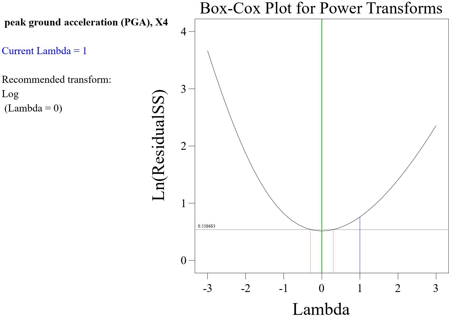
The Box-Cox plot presented in Figure 7 is a diagnostic tool used to identify an appropriate power transformation for the PGA(response variable) in this response surface model (RSM) or any other statistical model. The goal of the Box-Cox transformation is to stabilize the variance and make the data more closely approximate a normal distribution, thus meeting the assumptions of many statistical models. In a Box-Cox plot, the x-axis represents the values of lambda ($\lambda$), which is the power parameter used in the Box-Cox transformation. Lambda values are typically plotted within a range, often from -2 to 2, representing different potential transformations. On the y-axis, the plot typically displays a measure of the transformed data’s normality, such as the log-likelihood function or another suitable metric. This allows you to assess how well the data conforms to normality under different transformation scenarios. The goal of the Box-Cox plot illustrated in Figure 7 is to identify the lambda value that maximizes the normality of the transformed data. This is often indicated by the lambda value that corresponds to the peak or plateau in the plot (see Figure 8), where the transformed data best approximates a normal distribution. When interpreting the Box-Cox plot, you should look for the lambda value that provides the best improvement in normality. A lambda of 0 represents a log transformation, and as the lambda value deviates from 0, it represents different power transformations. The plot helps in visualizing the impact of these transformations on the normality of the data. Once an appropriate lambda value is identified from the Box-Cox plot, the RSM model can be re-estimated using the transformed response variable. This can lead to improved model performance, especially if the original data exhibited issues such as heteroscedasticity or non-normality. In summary, the Box-Cox plot for power transform in an RSM model is used to identify an appropriate power transformation for the response variable, with the aim of improving the normality and variance properties of the data, thus enhancing the model’s performance.

Figure 8 RSM plot of predicted versus actual PGA values.

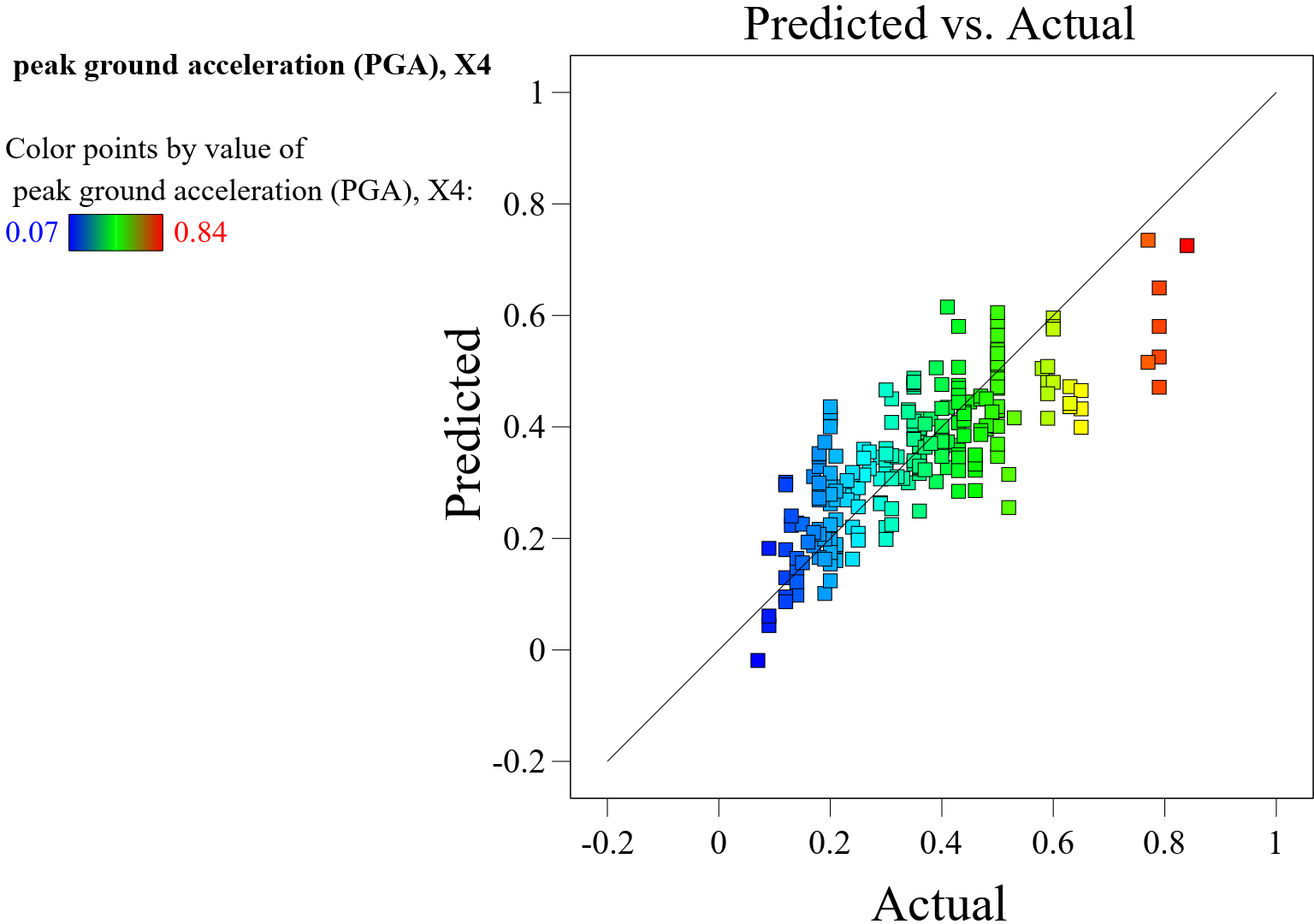
The Figure 8 displays an RSM plot of predicted versus actual Peak Ground Acceleration (PGA) values, where color points represent the magnitude of PGA from 0.07 to 0.84. Key observations and analysis are as follows: The data points are scattered around the diagonal reference line, indicating that the model has a reasonable alignment between predicted and actual PGA values. The closer the points are to this line, the more accurate the predictions. In the lower and middle ranges of PGA (blue to green points), the predictions generally cluster near the diagonal, demonstrating better accuracy. However, for higher PGA values (yellow to red points), the data points show more deviation, indicating potential prediction errors or model limitations in capturing extreme values. Deviations from the reference line, particularly in high-PGA regions, may point to the need for further model improvement or feature enhancement to handle higher magnitude predictions. The color gradient shows a gradual transition across the predicted and actual axes, suggesting a continuous relationship between the predicted and actual PGA values without abrupt shifts. Some points, particularly in the higher PGA range (red points), are far from the diagonal, indicating instances where the model may have overestimated or underestimated PGA. This plot suggests that while the model performs reasonably well for moderate PGA values, further refinement or additional features may be required to enhance its performance for extreme PGA predictions.

Figure 9 RSM plot of residuals versus moment magnitude for PGA prediction.

Figure 10 RSM plot of leverage versus run in PGA prediction.

Figure 11 RSM plot of DFFITS versus run in PGA prediction.

Figure 12 RSM plot of DFBETAS for intercept versus run in PGA prediction.

Figure 13 RSM plot of the desirability of optimized PGA values from 100 solutions.

In a response surface model (RSM), a plot of predicted versus actual values illustrated in Figure 8 is a useful diagnostic tool for evaluating the model’s predictive performance and identifying potential discrepancies between the predicted values generated by the model and the actual observed values from the data. In an ideal situation, the predicted versus actual values plot would show a strong linear relationship, with the points falling close to the 45-degree line ($y=x$). This would indicate that the model’s predictions closely match the actual observed values. If the points on the plot deviate systematically from the 45-degree line, it suggests that the model may have biases or shortcomings in its predictive capabilities. For example, if the model consistently underestimates or overestimates the actual values across a range of predictions, this could indicate a systematic issue. The spread of the points around the 45-degree line can also provide insights into the variability of the model’s predictions. If the spread of points widens or narrows as the actual values increase, it may suggest issues with heteroscedasticity, where the variance of the errors is not consistent across the range of predictions, as shown in Figures 9, 10, 11, 12 and 13. The plot can help identify outliers or influential points that may have a large impact on the model’s predictive performance. Outliers may appear as points that deviate significantly from the expected pattern on the plot. Overall, the plot of predicted versus actual values serves as a valuable diagnostic tool for assessing the accuracy and reliability of the RSM model’s predictions. It helps in identifying potential model misspecification, biases, heteroscedasticity, and influential observations. In summary, the plot of predicted versus actual values in an RSM model provides insights into the model’s predictive performance, highlighting areas where the model’s predictions align well with the actual data and areas where improvements may be necessary.

4.2 Novelty and practical relevance

The RSM research model demonstrates novelty through its ability to comprehensively explore the relationships between multiple independent variables and response variables within complex systems, such as predicting Peak Ground Acceleration (PGA). By employing a structured experimental design combined with regression techniques, it offers a versatile platform for optimizing outcomes and understanding intricate interactions among parameters. A significant aspect of its practical relevance is its potential for real-world problem-solving in geotechnical and seismic applications. The model allows researchers and engineers to develop predictive frameworks capable of improving structural resilience by accurately forecasting seismic behaviors. The capacity of RSM to visualize trends, optimize operating conditions, and provide solutions with minimized experimentation makes it a valuable tool for resource-efficient analysis. Additionally, integrating desirability functions enables multi-objective optimization, allowing stakeholders to balance competing performance criteria such as cost, safety, and sustainability. This versatility makes the RSM model an innovative and indispensable approach to enhancing decision-making processes in infrastructure development and geophysical flow predictions.