Chinese Journal of Information Fusion
ISSN: 2998-3371 (Online) | ISSN: 2998-3363 (Print)
Email: [email protected]


In recent years, due to the continuous global warming [1, 2], the sea ice in high-latitude regions has been persistently melting [3, 4]. The resulting high-latitude waterways can shorten the sailing distances between major trading powers and are urgently in need of development as future maritime routes [5, 6, 7]. Specifically, sea ice detection has always been the focus of research in high-latitude seas, which is devoted to accurately locating the positions of sea ice and identifying the scales of sea ice [8, 9].
A multitude of technologies are emerging in the domain of real-time object detection. They are extensively adopted in diverse industries, including the identification of suspicious behavior [10], the detection of anomalies in medical images [11], and fish detection [12], and other applications. In recent years, researchers have been concentrating on designing CNN-based object detectors [13, 14, 15, 16, 17, 18]. Among them, YOLOs achieve accurate classification and positioning of objects with low latency, and they are increasingly gaining popularity [19, 20, 21, 22, 23, 24, 25, 26, 27].
Furthermore, for an extended period, considerable efforts have been directed towards obtaining high-quality sea ice satellite remote sensing information and detecting sea ice from a diverse range of satellite remote sensing data [28, 29, 30, 31]. Hu et al. [32] detected sea ice using GNSS bidirectional radar reflections, where the local linear embedding (LLE) algorithm was employed for sea ice feature extraction. Liu et al. [33] proposed a Bayesian method with consideration of geometric characteristics of China France Oceanography Satellite scatterometer(CSCAT) for sea ice detection. The method operationally produced daily polar sea ice mask throughout its mission duration from 2019 to 2022. Jafari et al. [34] developed an automated method for iceberg detection and classification in complex sea conditions. Using the RADARSAT Constellation Mission (RCM), they collected seasonal sea ice data from the east coast of Canada.
To obtain more abundant spectral information, researchers have explored diverse types of optical remote sensing data [35, 36, 37, 38]. Researchers have focused on studying sea ice with visible remote sensing data, as the human eye can intuitively perceive the difference between sea ice and seawater in the visible wavelength band. Advancements in deep convolutional neural networks have achieved automated sea ice detection using visible remote sensing data. Ding et al. [39] proposed a detection model based on YOLOv5. They added Squeeze-and-Excitation Networks (SE) [40] to backbone of YOLOv5. The SE module computes channel-wise attention weights through global average pooling and multilayer perceptron, which are then applied to recalibrate feature map channels by element-wise multiplication. However, over-dependence on channel attention mechanisms (e.g., SE) inevitably discards spatially fine-grained features in imagery, particularly ice-water interface textures and areal extent variations that are critical for sea ice detection.
In this paper, we aim to address these questions precisely and further broaden the application scope of YOLOs. Refining the details of YOLOv8, we aim to enhance its capability in identifying sea ice across a variety of sizes.
Our contributions are as follows:
First, we propose a fusion module based on the attention mechanism and use it to replace the Concat module in the YOLOv8 network structure. This module can effectively help YOLOv8 extract the characteristic information of sea ice.
Second, we conduct an applicability analysis of the bounding box regression loss function in YOLOv8 and ultimately select Shape-IoU, which is more suitable for sea ice, as the loss function for bounding box regression. YOLOv8 utilizing Shape-IoU [41] not only demonstrates superior detection accuracy across all three categories of sea ice, but it also significantly reduces convergence time.
Third, we analyze the distribution characteristics of sea ice with different sizes in the NWPU-RESISC45 dataset. Based on these distribution characteristics, the bounding box information predicted by YOLOv8 are converted into evidence vectors for uncertainty quantification. Subsequently, evidence fusion [42] is achieved by fusing these vectors with the probability of sea ice categories.
Based on Landsat-8 satellite data, we have created a sea ice dataset and made it publicly available on this website: https://github.com/LiuYang0911/A-Proprietary-Visible-Light-based-Sea-Ice-Dataset.
By comparing with current mainstream object detection algorithms, our improved YOLOv8 achieves better detection accuracy and faster convergence speed.
We are optimistic that the outcomes of our efforts can act as a catalyst for the progress of fellow researchers in this domain.
Initially, attention mechanisms were utilized in machine translation tasks. This mechanism enables the model to focus on different parts of the input sentence when translating a word, which significantly enhances the translation quality [43]. Over the past years, considerable efforts have been devoted to developing attention mechanism modules that are more applicable to the domain of computer vision [40, 44, 45].
Channel attention mechanism: This type of attention mechanism, which concentrates on the channel dimension of the feature map, aims to enhance significant channel information while suppressing less important data. It accomplishes this by learning weights for each channel, akin to the methodology employed in SENet [40]. In SENet [40], the input feature map is first compressed along the spatial dimension before calculating weights for each channel. Finally, these weights are applied to multiply with the input feature map to produce the final output.
Spatial attention mechanism: In contrast to the channel attention mechanism, the spatial attention mechanism emphasizes the locations of valid information within the feature map, as exemplified by STN [44]. STN [44] is capable of extracting characteristics from significant regions across various deformation data to produce final prediction results.
Hybrid Attention Mechanism: Compared to the aforementioned two attention mechanisms, this particular attention mechanism comprehensively leverages both channel information and spatial information from feature maps, as exemplified by CBAM [45]. It sequentially employs the channel attention module followed by the spatial attention module to generate attention weights, ultimately producing the final feature map.
In 2016, Joseph Redmon introduced YOLOv1 [18], a real-time object detector built upon the deep learning framework Darknet. When compared to other object detectors [13, 14, 15, 16, 17], YOLOs [18, 19, 20] demonstrate superior detection performance while maintaining high detection speeds.
Over the past few years, significant efforts have been dedicated to exploring more efficient modules and network architectures for the YOLO series. YOLOv4 [21] and YOLOv5 [22] investigated the impact of various activation functions on detection accuracy and speed. It is essential to recognize that YOLOv5 [22] has been widely adopted across numerous sectors as a highly effective object detector. Building upon RepVGG, YOLOv6 [23] introduced RepBlock to replace the CSPDarknet53 [46] architecture used in YOLOv5, which allows the model to better integrate multi-scale features. Furthermore, based on YOLOv5 [22], YOLOv7 [24] proposed E-ELAN [47], which enhances the network's learning capability while preserving the original gradient path.
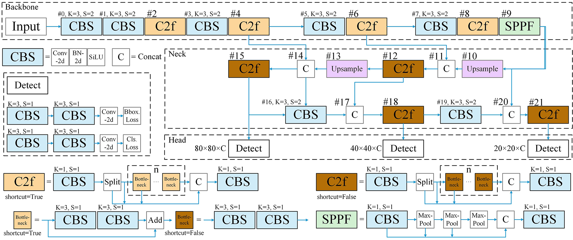
Based on the C3 module of YOLOv5 [22], YOLOv8 [25] has developed the C2f module, as illustrated in Figure 1. This module dynamically adjusts the number of channels according to the model's size, enabling it to flexibly adapt to various scenarios.
YOLOv9 [26] introduced G-ELEN, a network architecture that integrates the features of CSPNet [46] and ELEN [47], aiming to enhance detection accuracy while preserving detection speed. Building on the foundation established by YOLOv8 [25], YOLOv10 [27] presented several improvements, including the use of classification heads with reduced parameters and the incorporation of a partial self-attention module, etc., all designed to further transcend the accuracy-speed trade-offs inherent in YOLO models.
The object detector based on convolutional neural networks employs a loss function to update the network weights [48]. Historically, iterations of the YOLO object detectors have been engaged in an unrelenting pursuit of optimizing the loss function for bounding box regression, aiming to achieve superior performance [48, 49, 50]. Simultaneously, a variety of loss functions for boundary box regression are continuously being developed and refined [41, 51, 52, 53, 54], thereby enabling the improved YOLOv8-based object detector to be applied across an increasingly diverse range of scenarios.
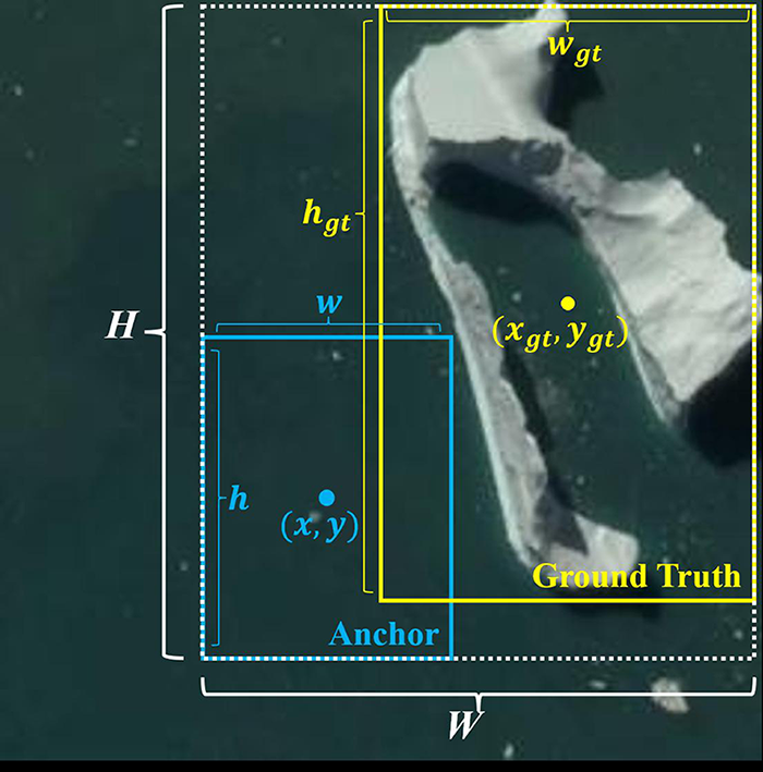
The YOLOv8 model employs C-IoU [50] as the loss function for bounding box regression, as shown in Figure 2. The following presents the mathematical expression for C-IoU [50]:
From the formulas, it is evident that C-IoU [50] takes into account both the position and shape of the bounding box in a comprehensive manner. This allows the model to learn the characteristics of the ground truth box more thoroughly.
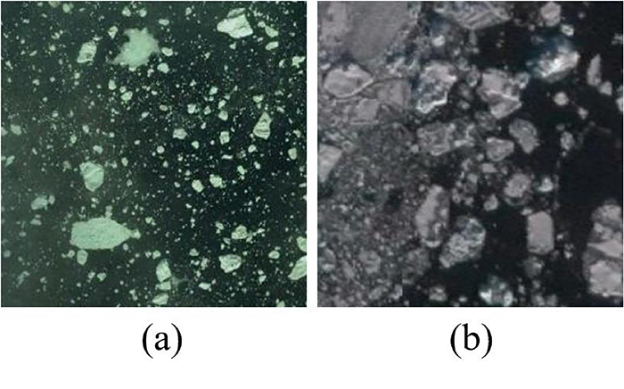
We categorize these sea ice instances into three distinct groups, as elaborated in section 4.1. Although satellite imagery offers relatively high resolution, actual ice conditions can be highly complex. As shown in Figure 3, several factors make it challenging for object detection models to accurately identify sea ice of varying scales. These include the wide range of ice floe sizes, irregular shapes, and reduced contrast between ice and seawater caused by melting and accumulation of sea ice.
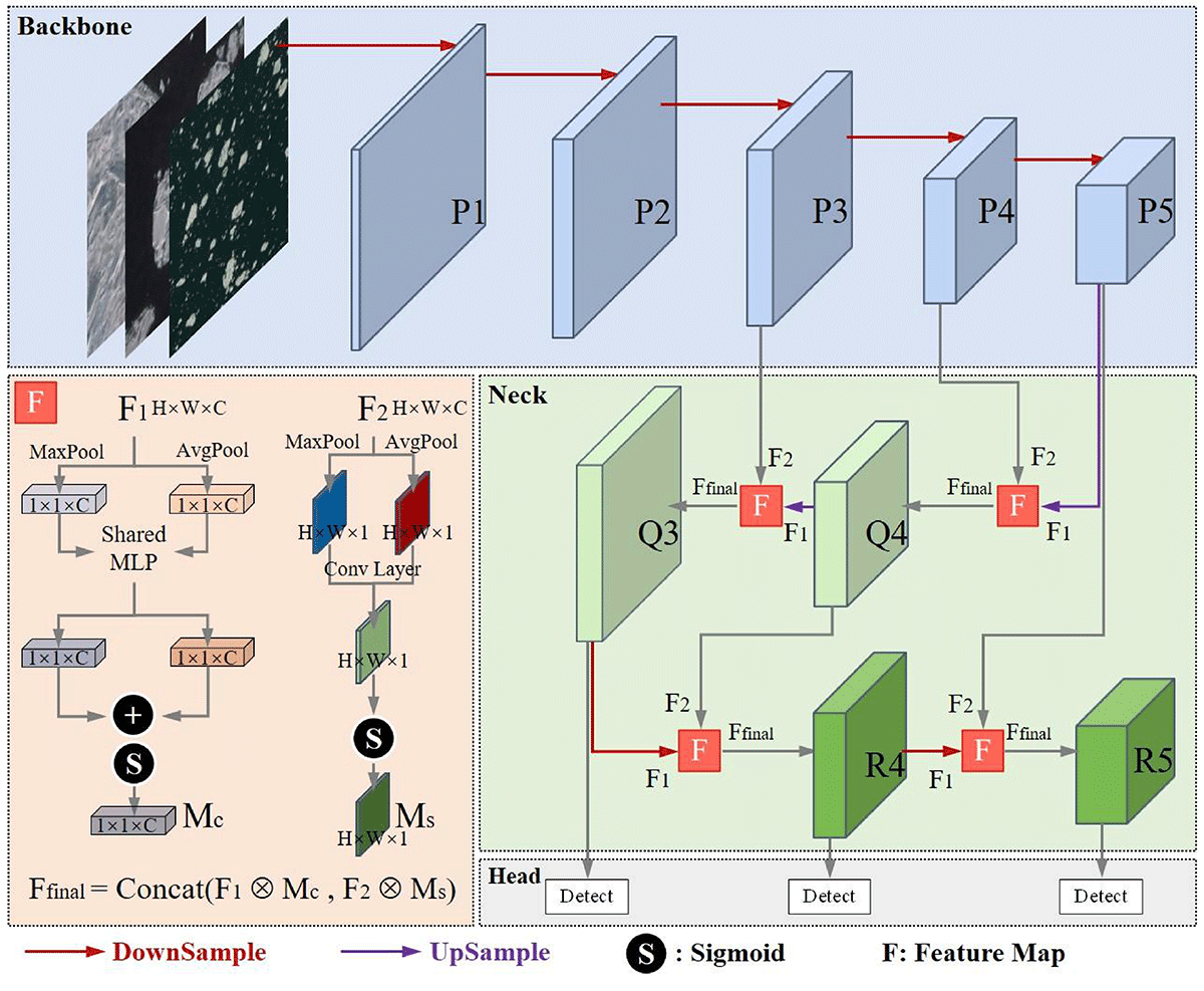
Besides, as the network deepens, the detection model progressively enhances semantic information in feature maps while inevitably sacrificing spatial details, particularly size characteristics crucial for sea ice analysis. When handling this task, YOLOv8 uses the Concat module to combine deep and shallow feature maps. However, we observe that relying on the feature maps after direct stitching is not sufficient for accurate size classification. To address this limitation, we propose an attention-based fusion module that can effectively enhance the spatial detail information in the feature map, so as to be able to accurately distinguish between sea ice size categories, as shown in Figure 4.
First, we calculate the channel attention weight of the feature map and multiply it with the feature map to obtain . Secondly, we calculate the Spatial attention weights of the feature map and multiply it with the feature map to obtain . Thirdly, we concatenate the feature map and to obtain the final feature map . The detailed process is as follows:
where the feature map is derived from deeper layers and contains more semantic information, such as the overall shape and categories of sea ice; the feature map is derived from shallower layers and includes more detailed information, such as edges, textures, colors, and other low-level features of sea ice. In this way, we optimize the fusion process of different feature maps in YOLOv8, enabling the model to balance attention between the semantic information and detailed information of different feature maps, thereby improving the detection accuracy of the model for sea ice of varying scales.
The C-IoU loss [50] employed in YOLOv8 considers the geometric relationship between the ground truth box and the predicted box, utilizing both their relative positions and shapes to compute the loss. However, in contrast to general objects, sea ice presents a more diverse aspect ratio and possesses an irregular shape that lacks any fixed pattern. In this study, if C-IoU [50] is utilized as the loss function for bounding box regression, two critical questions arise.
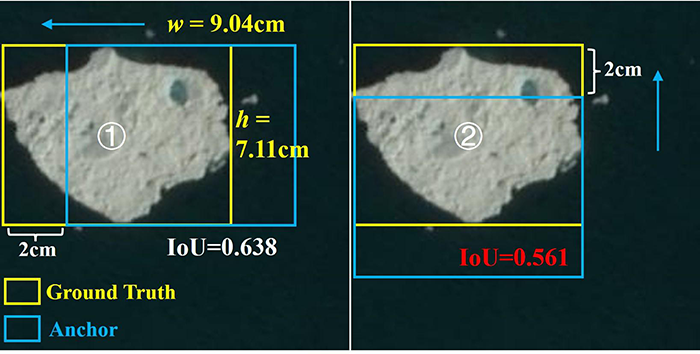
As shown in Figure 5, targets \scriptsize1⃝ and \scriptsize2⃝ represent the same sea ice. When two bounding boxes exhibit the same absolute deviation from the ground truth box, the bounding box that regresses from the direction of the shorter side of the rectangle tends to demonstrate a lower Intersection over Union (IoU) value. Our research indicates that this variation in IoU is more pronounced when regression occurs from the direction of the shorter side during bounding box adjustment. Consequently, it is crucial for models to effectively balance the regression impact of bounding boxes originating from different directions.
As illustrated in Figure 6, the center points of the prediction boxes \scriptsize3⃝ and \scriptsize4⃝ have shifted closer to the position of the ground truth box. Furthermore, both prediction boxes maintain an equal distance from the ground truth box along both the long and short sides. However, it is noteworthy that target \scriptsize4⃝, which regressed from the short side, corresponds to a lower IoU value, indicating reduced overlap with the ground truth.
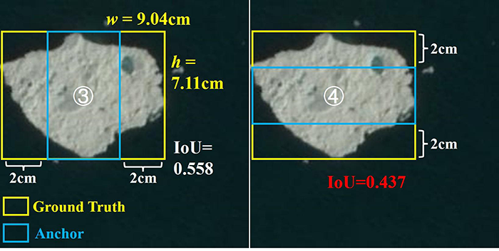
During the bounding box regression process, the variation in IoU is particularly significant when the regression occurs along the short side of the ground truth box. Therefore, it is essential to ensure a balanced regression effect for bounding boxes across various directions throughout this process.
In the end, we select Shape-IoU [41] as our loss function for bounding box regression, as it effectively addresses the two types of issues mentioned above. The formula for Shape-IoU [41] is presented below:
where represents the scale factor, which can be adjusted based on the dimensions of the target. Taking the ground truth box in Figure 5 as an example(where ), when and , the bounding box regression lacks directional prioritization. by increasing the value of scale, the regression effectiveness can be enhanced. In this study, we set , resulting in , which indicates that higher regression weight is assigned to the vertical dimension (height adjustment).
Equation 10 calculates the loss value for bounding box regression.
It is noteworthy that Shape-IoU dynamically emphasizes the gradient update path of bounding box parameters (e.g., center offsets and aspect ratios) during model convergence. Unlike C-IoU, which indirectly guides optimization through geometric penalties (center distance and aspect ratio matching), Shape-IoU explicitly introduces a directional weighting coefficient, thereby clarifying the prioritization of regression targets with higher shape discrepancies. This property of Shape-IoU shortens the convergence time of the model.
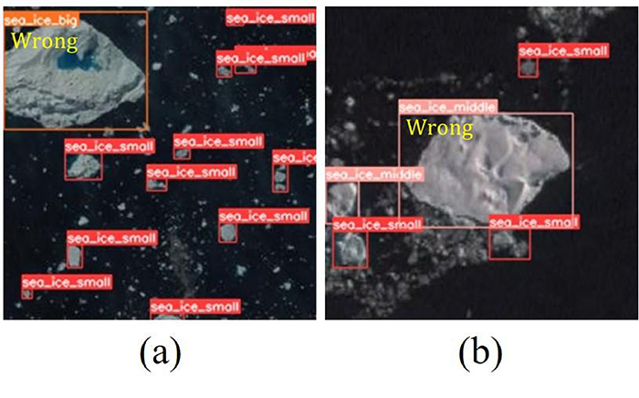
After extensive experimentation, we discovered that YOLOv8 is capable of accurately predicting the bounding boxes of sea ice; however, it occasionally misclassifies the categories of sea ice. More specifically, YOLOv8 occasionally misclassifies medium-scale sea ice as large-scale sea ice and conversely misclassifies large-scale sea ice as medium-scale sea ice, As illustrated in Figure 7.
In Figure 7 (a), the sea ice located in the upper left corner is classified as medium-scale, as the longest side of its circumscribed rectangle measures less than 128 pixels. However, it was incorrectly identified by YOLOv8 as large sea ice. Meanwhile, in Figure 7 (b), the sea ice situated at the center is categorized as large-scale, given that the longest side of its circumscribed rectangle exceeds 128 pixels. However, it was inaccurately classified by YOLOv8 as medium-scale sea ice.
With these issues in consideration, we conducted a more thorough examination of YOLO. The YOLO algorithm is designed to extract features from images and classify targets based on these extracted characteristics. The features encompass various types of information, including texture, color, shape, and more. More specifically, YOLO relies more heavily on the aforementioned features for target classification than on the scale information of the targets.
However, in our task of classifying sea ice, the scale information of the target cannot be overlooked. We aim to improve YOLOv8 so that the scale information of the target can serve as a more significant feature for predicting categories of sea ice.
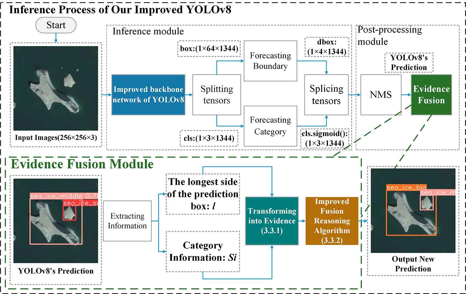
In the inference process of YOLOv8, the role of non-maximum suppression (NMS) is to eliminate redundant prediction boxes and produce the final output. Based on this, we propose the Evidence Fusion module to address the aforementioned issues, the details of the Evidence Fusion module are illustrated in Figure 8.
First, we convert the prediction box information and prediction category information provided by YOLOv8 into evidences. Utilizing an enhanced DSmT fusion inference algorithm [42], we subsequently integrate these two types of evidence to establish a new prediction category. The algorithmic model is primarily composed of the following two components.
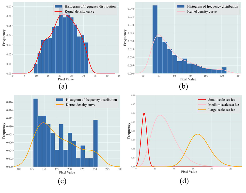
The bounding box information predicted by YOLOv8: We begin by counting the instances of sea ice larger than 8 pixels in the satellite image dataset NWPU-RESISC45 [29]. Subsequently, we categorize these sea ice instances into three distinct groups based on their scale, as elaborated in section 4.1. Finally, we generate histograms to illustrate the frequency distribution of the longest side of the circumscribed rectangles for each type of sea ice and fit distribution curves to these histograms, as depicted in Figure 9.
small.png)
medium.png)
big.png)
The category information predicted by YOLOv8: The prediction values for the three types of sea ice—clssmall, clsmedium, clslarge—are included in the prediction information provided by YOLOv8. The category with the highest prediction value indicates the model's predicted target. We convert this set of data into category evidence, as shown in equations 15.
small.png)
medium.png)
big.png)
| Small-Scale Sea Ice | Medium-Scale Sea Ice | Big-Scale Sea Ice | ||
| NWPU- RESISC45 [29] | Quantity | 6820 | 3710 | 382 |
| Percentage | 62.5% | 34.0% | 3.5% | |
| Our Sea Ice Dataset | Quantity | 3162 | 1170 | 256 |
| Percentage | 69.0% | 25.5% | 5.5% | |
| Note: We randomly select 70% of the images to train the model, and the remaining 30% of the images were used to verify the training effect. | ||||
| Attribute | Attribute Value | |||||
| 1 | 2 | |||||
| SPACECRAFT_ID | LANDSAT8 | LANDSAT8 | ||||
| ORIGIN |
|
|
||||
| LANDSAT_SCENE_ID | LC80482392019215LGN00 | LC81300082018179LGN00 | ||||
| LANDSAT_PRODUCT_ID |
|
|
||||
| FILE_DATE | 2019-08-19T23:27:47Z | 2018-07-04T09:14:55Z | ||||
| OUTPUT_FORMAT | GEOTIFF | GEOTIFF | ||||
| SENSOR_ID | OLI_TIRS | OLI_TIRS | ||||
| TARGET_WRS_PATH | 48 | 130 | ||||
| TARGET_WRS_ROW | 239 | 8 | ||||
| DATE_ACQUIRED | 2019-08-03 | 2018-06-28 | ||||
| SCENE_CENTER_TIME | 20:32:39.0212890Z | 03:26:15.2127540Z | ||||
| CLOUD_COVER | 1.55 | 2.20 | ||||
| CLOUD_COVER_LAND | 0.02 | 0.12 | ||||
| IMAGE_QUALITY_OLI | 9 | 9 | ||||
| IMAGE_QUALITY_TIRS | 9 | 9 | ||||
| Note: This dataset pertains to the sea ice data corresponding to the aforementioned two scenes. The dataset comprises a total of 430 images, each with dimensions of 256 * 256 pixels. | ||||||
| Attribute | Attribute Value |
| CPU | Core i5 12450H |
| GPU | NVIDIA GeForce RTX 3050 |
| Running memory | 16GB |
| Storage memory | 256GB |
| Operating system | Win 10 |
| Interpreter | Python 3.9 |
| Deep Learning Frameworks | PyTorch 1.9 |
| IDEA | PyCharm |
| Attribute | Attribute Value |
| epochs | 500 |
| batch size | 16 |
| imgsz | 256 |
| workers | 8 |
| close mosaic | Last 10 epochs |
| optimizer | AdamW |
| initial learning rate | 0.01 |
| final learning rate | 0.0001 |
| momentum | 0.937 |
| weight decay | 0.0005 |
| warm-up epochs | 3.0 |
| warm-up momentum | 0.8 |
| warm-up bias learning rate | 0.1 |
| box loss gain | 7.5 |
| class loss gain | 0.5 |
| DFL loss gain | 1.5 |
| hsv hue augmentation | 0.015 |
| hsv saturation augmentation | 0.7 |
| hsv value augmentation | 0.4 |
| translation augmentation | 0.1 |
| scale augmentation | 0.9 |
| mosaic augmentation | 1.0 |
| mixup augmentation | 0.1 |
| copy-paste augmentation | 0.1 |
| Model | Precision (%) | Recall (%) | mAP50 (%) | mAP50-95 (%) | F1 (%) | Training time (h) | FPS |
| Faster R-CNN | 62.7 | 80.3 | 79.2 | 47.1 | 70.4 | 6.09 | 4.4 |
| SSD | 62.3 | 76.0 | 78.0 | 47.6 | 68.5 | 0.98 | 6.9 |
| RT-DETR | 74.9 | 66.1 | 73 | 54.2 | 70.2 | 3.213 | 68.0 |
| YOLOv3 | 66.8 | 86 | 74.7 | 50.9 | 75.2 | 5.719 | 59.2 |
| YOLOv5 | 73.3 | 73.3 | 82.2 | 52.5 | 73.3 | 0.728 | 208.3 |
| YOLOv6 | 72.4 | 69.3 | 78.4 | 47.0 | 70.8 | 3.262 | 69.4 |
| YOLOv7 | 76.7 | 64.6 | 81.5 | 49.1 | 70.1 | 4.529 | 87.7 |
| YOLOv9 | 65.6 | 82.3 | 78.0 | 44.2 | 73.0 | 5.46 | 108.7 |
| YOLOv10 | 84.2 | 68.1 | 81.9 | 49.0 | 75.3 | 0.483 | 128.2 |
| ASF-YOLO | 64.6 | 77.9 | 80.3 | 45.1 | 70.6 | 3.983 | 53.5 |
| GOLD-YOLO | 73.4 | 74.7 | 81.1 | 47.8 | 74.0 | 6.118 | 58.5 |
| Hyper-YOLO | 69.2 | 76.9 | 83.1 | 50.5 | 72.8 | 6.307 | 44.4 |
| Improved YOLOv5[39] | 71.2 | 75.1 | 82.6 | 51.5 | 73.1 | 3.52 | 126.4 |
| YOLOv8 | 84.7 | 62.4 | 81.6 | 56.2 | 71.9 | 1.113 | 82.6 |
| Our Improved YOLOv8 | 79.4 | 78.0 | 87.2 | 59.3 | 78.7 | 0.959 | 48.3 |
| In the same group of experiments, the best-performing data is highlighted in bold. | |||||||
We currently employ two distinct sea ice datasets to assess the detection accuracy of our improved YOLOv8 model. The first dataset is the widely recognized NWPU-RESISC45 [29], while the second consists of an exclusive Landsat8-based sea ice dataset that we have developed.
When traversing sea-ice laden waters, it is imperative for the crew to swiftly discern and precisely locate sea ice of diverse dimensions to enable the vessel to bypass the perilous sea ice. Consequently, we categorize the sea ice in these two datasets into three distinct categories. We employ the software labelimg [55] to annotate the images of three distinct types of sea ice, designated as Small-scale sea ice, Medium-scale sea ice, and Large-scale sea ice, as shown in Figure 10.
We cropped the satellite data into uniformly sized images and utilized the software labelimg [55] to annotate three distinct types of sea ice present in these images, designated as Small-scale sea ice, Medium-scale sea ice, and Large-scale sea ice, as shown in Figure 11. The specifics of this dataset are provided in the appendix, as shown in Tables 1 and 2.
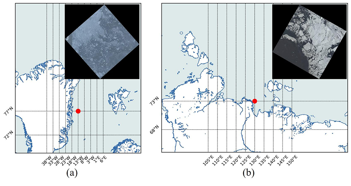
In addition to the NWPU-RESISC45 [29] dataset, we also explored other datasets to continually validate the performance of our enhanced YOLOv8-based sea ice detector. We identified areas where sea ice occurs at high latitudes and acquired satellite data for these regions, as depicted in Figure 12.
| Model | Precision (%) | Recall (%) | mAP50 (%) | mAP50-95 (%) | F1 (%) | Training time (h) | FPS |
| Faster-RCNN | 70.7 | 84.1 | 83.2 | 66.2 | 76.8 | 14.79 | 5.8 |
| SSD | 72.1 | 71.4 | 72.0 | 53.5 | 71.7 | 2.38 | 6.9 |
| RT-DETR | 66.7 | 67.2 | 73.6 | 45.4 | 66.9 | 7.871 | 40.5 |
| YOLOv3 | 73.1 | 71.3 | 81.4 | 50.2 | 72.2 | 6.29 | 53.8 |
| YOLOv5 | 72.5 | 88.9 | 90.2 | 69.5 | 79.9 | 2.499 | 156.4 |
| YOLOv6 | 74.0 | 77.0 | 80.4 | 46.1 | 75.5 | 13.668 | 52.8 |
| YOLOv7 | 74.9 | 74.6 | 82.8 | 53.0 | 74.7 | 2.142 | 192.3 |
| YOLOv9 | 86.8 | 70.3 | 84.7 | 52.8 | 77.7 | 1.921 | 181.8 |
| YOLOv10 | 77.5 | 91.6 | 91.3 | 62.2 | 84.0 | 1.581 | 112.8 |
| ASF-YOLO | 77.3 | 90.0 | 91.6 | 68.5 | 83.2 | 5.865 | 61.7 |
| GOLD-YOLO | 81.7 | 65.9 | 82.1 | 51.6 | 73.0 | 6.919 | 55.6 |
| Hyper-YOLO | 86.2 | 66.4 | 86.3 | 55.0 | 75.0 | 8.5 | 70.9 |
| Improved YOLOv5[39] | 75.1 | 90.3 | 90.1 | 65.9 | 82.0 | 2.042 | 134.7 |
| YOLOv8 | 86.1 | 85.6 | 92.7 | 67.6 | 85.8 | 9.435 | 50.8 |
| Our Improved YOLOv8 | 90.6 | 78.0 | 93.8 | 71.8 | 87.4 | 4.624 | 53.2 |
| In the same group of experiments, the best-performing data is highlighted in bold. | |||||||
We use YOLOv8 as a baseline model. Since the release of YOLOv8 in 2023, it has been deployed on various types of hardware due to its low resource requirements. The following are the experimental configuration, hyper-parameters of improved YOLOv8 object detector and summary of the labels for the three types of sea ice, as shown in Tables 3 and 4.


As shown in Table 5, we conduct experiments on the NWPU-RESISC45 Dataset with mainstream object detection algorithms and perform a comparative analysis of our improved YOLOv8. The selected object detection algorithms include: the two-stage object detection algorithm Faster R-CNN, the Transformer-based object detection algorithm RT-DETR, the one-stage object detection algorithms from the YOLO series, and the improved YOLO series algorithms. Compared to YOLOv8, our improved YOLOv8 achieves a 15.6% increase in Recall, a 5.6% improvement in mAP50, a 3.1% enhancement in mAP50-95, and a 6.8% boost in F1 score, while simultaneously reducing the training time by 13.8%.
In addition, compared to other improved YOLO series algorithms, our enhanced YOLOv8 also demonstrates outstanding detection accuracy and relatively faster convergence speed. As Figure 13 illustrates, we present the detection effects of our improved YOLOv8 alongside the baseline model YOLOv8.
| Dataset | Method | Fusion Module | Shape-IoU | Evidence Fusion | mAP50 (%) | mAP50-95 (%) |
| NWPU-RESISC45 [29] | YOLOv8 | 81.6 | 56.2 | |||
| Algorithm 1 | 83.3 | 57.0 | ||||
| Algorithm 2 | 82.8 | 58.3 | ||||
| Algorithm 3 | 85.3 | 56.8 | ||||
| Our Improved YOLOv8 | 87.2 | 59.3 | ||||
| Our Sea Ice Dataset | YOLOv8 | 92.7 | 67.6 | |||
| Algorithm 1 | 92.9 | 68.2 | ||||
| Algorithm 2 | 93.2 | 70.1 | ||||
| Algorithm 3 | 93.3 | 68.0 | ||||
| Our Improved YOLOv8 | 93.8 | 71.8 | ||||
| Note: denotes an added module based on YOLOv8. In the same group of experiments, the best-performing data is highlighted in bold. | ||||||
| Dataset | Method | AP50(%) | mAP50 (%) | mAP50-95 (%) | |||
| small | medium | big | |||||
| NWPU-RESISC45 [29] | YOLOv8 | 80.3 | 80.8 | 83.7 | 81.6 | 56.2 | |
| + SE | 52.3 | 87.2 | 88.3 | 75.9 | 51.7 | ||
| + EMA | 69.0 | 78.9 | 81.3 | 76.4 | 48.0 | ||
| + CA | 62.0 | 74.7 | 76.2 | 71.0 | 52.2 | ||
| + CBAM | 79.5 | 76.1 | 83.9 | 79.8 | 53.5 | ||
|
84.5 | 81.0 | 84.4 | 83.3 | 57.0 | ||
| Our Sea Ice Dataset | YOLOv8 | 89.1 | 94.0 | 95.0 | 92.7 | 67.6 | |
| + SE | 79.7 | 91.8 | 93.2 | 88.2 | 65.6 | ||
| + EMA | 84.4 | 91.1 | 92.2 | 89.3 | 60.3 | ||
| + CA | 85.9 | 91.8 | 94.3 | 90.7 | 66.7 | ||
| + CBAM | 80.9 | 89.3 | 91.3 | 87.2 | 64.4 | ||
|
89.3 | 94.1 | 95.3 | 92.9 | 68.2 | ||
| In the same group of experiments, the best-performing data is highlighted in bold. | |||||||
As shown in Table 6, we conduct experiments on the landsat 8-based sea ice dataset with mainstream object detection algorithms and perform a comparative analysis of our improved YOLOv8. The selected object detection algorithms include: the two-stage object detection algorithm Faster R-CNN, the Transformer-based object detection algorithm RT-DETR, the one-stage object detection algorithms from the YOLO series, and the improved YOLO series algorithms. Compared to YOLOv8, our improved YOLOv8 achieves a 4.5% increase in Precision, a 1.1% improvement in mAP50, a 4.2% enhancement in mAP50-95, and a 1.5% boost in F1 score, while simultaneously reducing the training time by 51.0%.
In addition, compared to other improved YOLO series algorithms, our enhanced YOLOv8 also demonstrates outstanding detection accuracy and relatively faster convergence speed. As Figure 14 illustrates, we present the detection effects of our improved YOLOv8 alongside the baseline model YOLOv8.


As shown in Table 7, we exhibit the results of ablation experiments based on our improved YOLOv8. On the basis of YOLOv8, we replace the Concat module with a fusion module to obtain Algorithm 1, we substitute the C-IoU with Shape-IoU to obtain Algorithm 2, and we add an evidence fusion module to obtain Algorithm 3.
The experimental data from the NWPU-RESISC45 dataset reveal that our improved network architecture, incorporating a fusion module, improves the mAP50 of YOLOv8 by 1.7%. In addition, we propose an evidence fusion module that improves the mAP50 of YOLOv8 by 3.7%. The experimental data from Our Sea Ice Dataset reveal that our improved network architecture, incorporating a fusion module, improves the mAP50 of YOLOv8 by 0.2%. In addition, we propose an evidence fusion module that improves the mAP50 of YOLOv8 by 0.6%.
As depicted in Table 8, we present the outcomes of the ablation experiments conducted on YOLOv8, utilizing various mainstream attention mechanisms.
As shown in Table 8, the attention module affects the detection accuracy improvement of YOLOv8, while the fusion module compensates for the negative impact of using only the attention mechanism and enhances the overall detection performance.
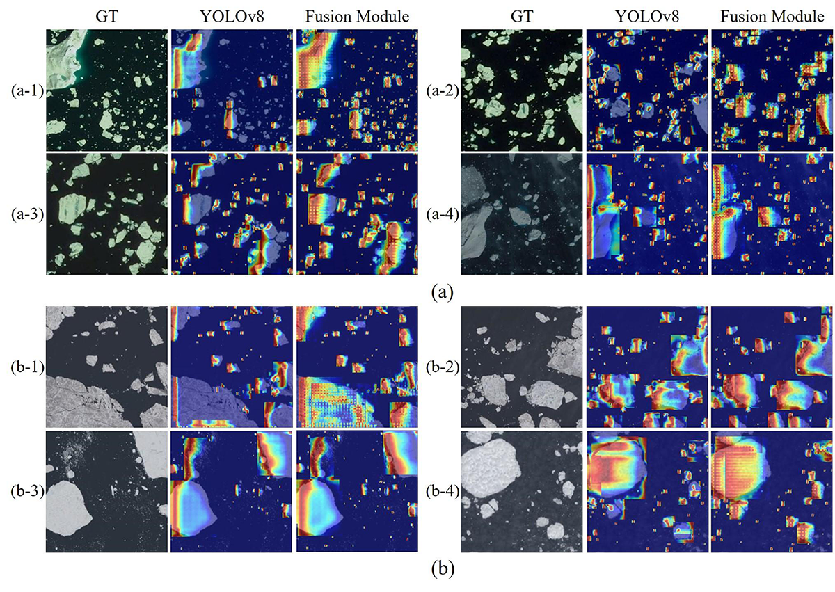
To intuitively perceive the positive impact of the fusion module, we use heatmaps to visualize the feature extraction effects of YOLOv8 after introducing our fusion module, as shown in Figure 15. Among them, Figure 15 (a) shows the experimental results of our improved YOLOv8 on the NWPU-RESISC45 dataset, while Figure 15 (b) presents the experimental results of our improved YOLOv8 on our sea ice dataset.
We substitute the C-IoU [50] loss with a contemporary mainstream loss function for bounding box regression. As demonstrated in Table 9, we present the results of ablation experiments conducted using YOLOv8.
| Dataset | Method | AP50(%) | mAP50 (%) |
|
|
||||||
| small | medium | big | |||||||||
| NWPU-RESISC45 [29] | YOLOv8 (C-IoU) | 80.3 | 80.8 | 83.7 | 81.6 | 56.2 | 1.113 | ||||
| + G-IoU | 72.5 | 75.9 | 77.8 | 75.4 | 53.1 | 1.058 | |||||
| + D-IoU | 72 | 72.9 | 75.3 | 73.4 | 56.2 | 1.710 | |||||
| + F-IoU | 74 | 75.1 | 81.1 | 76.7 | 56 | 1.071 | |||||
| + S-IoU | 74.8 | 76 | 82.9 | 77.9 | 55.6 | 0.958 | |||||
| + W-IoU | 78.5 | 79.8 | 82 | 80.1 | 56.4 | 1.000 | |||||
| + Inner-IoU | 75.3 | 78.4 | 78.8 | 77.5 | 53.9 | 1.839 | |||||
|
82.3 | 81.4 | 84.7 | 82.8 | 58.3 | 0.848 | |||||
| Our Sea Ice Dataset | YOLOv8 (C-IoU) | 89.1 | 94.0 | 95.0 | 92.7 | 67.6 | 9.435 | ||||
| + G-IoU | 80.9 | 84.7 | 83.7 | 83.1 | 66.4 | 10.810 | |||||
| + D-IoU | 84.3 | 85.5 | 86 | 85.3 | 67.4 | 10.138 | |||||
| + F-IoU | 82.9 | 84.4 | 83 | 83.4 | 68 | 9.234 | |||||
| + S-IoU | 82 | 87 | 86.6 | 85.2 | 68.9 | 10.465 | |||||
| + W-IoU | 83.7 | 93.5 | 93 | 90.1 | 68.7 | 9.911 | |||||
| + Inner-IoU | 81.8 | 86.5 | 84.8 | 84.4 | 69 | 11.868 | |||||
|
84 | 96.2 | 99.5 | 93.2 | 70.1 | 8.325 | |||||
| Dataset | Method |
|
|
|
mAP50 (%) | mAP50-95 (%) | Training Time (h) | ||||||
| NWPU- RESISC45 [29] | YOLOv8 (C-IoU) | 80.3 | 80.8 | 83.7 | 81.6 | 56.2 | 1.113 | ||||||
|
83.9 | 84.5 | 87.5 | 85.3 | 56.8 | - | |||||||
| Our Sea Ice Dataset | YOLOv8 (C-IoU) | 89.1 | 94.0 | 95.0 | 92.7 | 67.6 | 9.435 | ||||||
|
89.7 | 94.5 | 95.7 | 93.3 | 68.0 | - |
As illustrated in Table 9, when compared to other enhanced methods, YOLOv8 utilizing Shape-IoU [41] not only demonstrates superior detection accuracy across all three categories of sea ice, but it also significantly reduces convergence time.
Compared to YOLOv8, our Algorithm 2, equipped with Shape-IoU, achieves 1.2% mAP50 improvement, 2.1% mAP50-95 improvement along with a reduction in training time of 23.8%, as validated by the NWPU-RESISC45 dataset. Furthermore, this YOLOv8 variant equipped with Shape-IoU realizes a 0.5% increase in mAP50 and a 2.5% rise in mAP50-95 while concurrently reducing training time by 11.8%, as confirmed by our sea ice dataset.
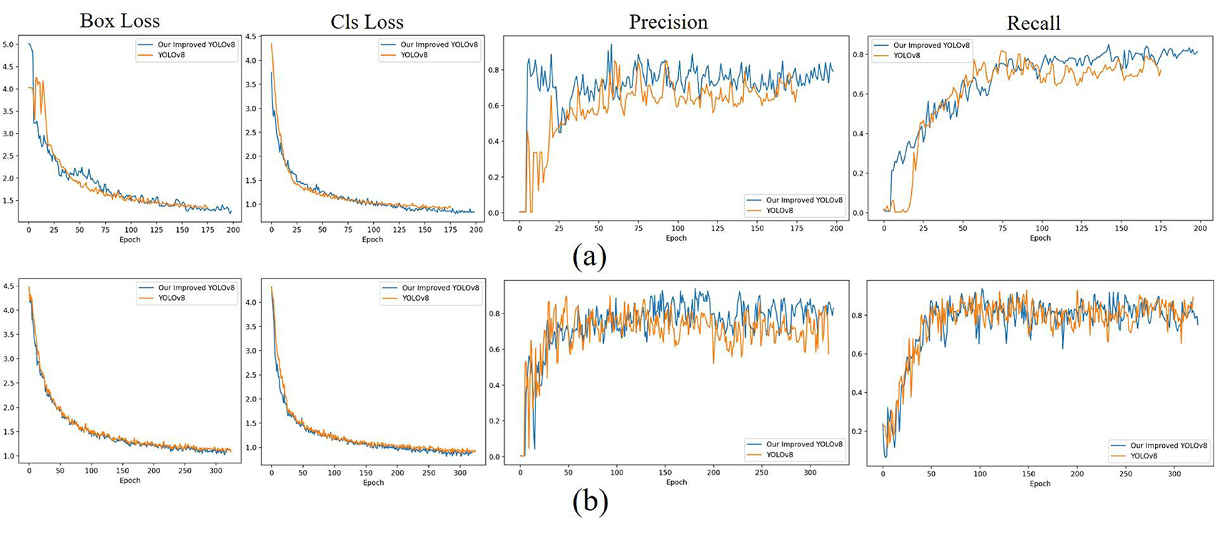
To intuitively perceive the positive impact of the Shape-IoU, we use Loss function curve to visualize the convergence process of our improved YOLOv8 and YOLOv8, as shown in Figure 16. Among them, Figure 16 (a) shows the convergence process of our improved YOLOv8 and YOLOv8 on the NWPU-RESISC45 dataset, while Figure 16 (b) presents the convergence process of our improved YOLOv8 and YOLOv8 on our sea ice dataset.
YOLOv8 utilizes a detection architecture which separates the tasks of classification and localization. This architecture disassembles the tensors, enabling independent predictions for both the bounding box and the category of each target.
The bounding boxes and categories of the targets in sea ice dataset are closely related. Consequently, the design of the detection architecture may result in inconsistencies between the predicted bounding boxes and their corresponding sea ice categories. For instance, a bounding box that represents large-scale sea ice might be inaccurately associated with a predicted category of medium-scale sea ice.
In summary, we simultaneously transform the bounding box and category information predicted by YOLOv8 into multiple pieces of evidence that characterize uncertainty. Subsequently, we utilize an enhanced DSmT fusion inference algorithm to predict the new category. As shown in Table 10, we exhibit the results of ablation experiments based on YOLOv8.
From Table 10, it is intuitively clear that YOLOv8, when using evidence fusion, achieves better detection accuracy on all three types of sea ice.
In this paper, we propose a YOLOv8-based sea ice detection algorithm designed to identify sea ice of various sizes in satellite imagery. Firstly, we incorporate an attention-based fusion module into the concatenation component of the YOLOv8 neck network. Secondly, we substitute the C-IoU loss function in YOLOv8 with the more recent Shape-IoU as the boundary regression loss for the detection head. Thridly, we convert the inference results of the YOLOv8's output into uncertain multiple evidences according to the size distribution of sea ice in the dataset. Subsequently, we fuse multiple pieces of evidences and infer new results based on the improved DSmT fusion inference algorithm. These bring our improved YOLOv8, an sea ice detection algorithm for detecting sea ice of multiple sizes in satellite imagery. The results show that our improved YOLOv8 achieves the state-of-the-art performance in two aspects: identifying sea ice and dividing sea ice size compared with the baseline model and other advanced detection algorithms.
 Copyright © 2025 by the Author(s). Published by Institute of Emerging and Computer Engineers. This article is an open access article distributed under the terms and conditions of the Creative Commons Attribution (CC BY) license (https://creativecommons.org/licenses/by/4.0/), which permits use, sharing, adaptation, distribution and reproduction in any medium or format, as long as you give appropriate credit to the original author(s) and the source, provide a link to the Creative Commons licence, and indicate if changes were made.
 Chinese Journal of Information Fusion
ISSN: 2998-3371 (Online) | ISSN: 2998-3363 (Print)
Email: [email protected]

Portico
All published articles are preserved here permanently:
https://www.portico.org/publishers/iece/